AMReX: from symbolic model to generated C++

AMReX: from symbolic model to generated C++#

AMReX is Zoomy’s block-structured adaptive-mesh backend. The model you write is the same one the NumPy tutorial uses — only the final step differs: instead of lambdifying into NumPy, the operators are printed as C++ and compiled against AMReX.

Before you start — you need the AMReX container#

This page does not stop at the generated code: it compiles it and runs the case. That needs the AMReX toolchain, which ships as a container:

# Apptainer (recommended)
apptainer pull zoomy_amrex.sif oras://ghcr.io/zoomylab/zoomy_amrex_sif:latest
apptainer run --bind $PWD:/workspace zoomy_amrex.sif jupyter
# -> open the printed http://127.0.0.1:8888/?token=... and run this notebook there

# Docker
docker run --rm -p 8888:8888 -v "$PWD:/workspace" \
    ghcr.io/zoomylab/zoomy_amrex:latest jupyter

See Installation for all containers and the three run modes. Nothing on this page needs a local AMReX build.

1. The model#

Identical to the NumPy tutorial — that is the point. Shallow water as SME(level=0), wall boundaries, dam-break initial state.

Two settings are AMReX’s, not the model’s. The structured grid names its boundaries West / East (plus South / North in 2-D), and the driver aborts on a tag it cannot find, so the BC tags carry those names. And symbolic_spectrum=True asks for the closed-form spectrum, which at level 0 is the ordinary shallow-water one and costs a couple of seconds — the emitted eigenvalue kernel is then the real spectrum rather than a numerical fallback.

import numpy as np

from zoomy_core.model.models import SME, Newtonian, NavierSlip, StressFree
import zoomy_core.model.boundary_conditions as BC
import zoomy_core.model.initial_conditions as IC

model = SME(
    level=0,
    symbolic_spectrum=True,
    closures=[Newtonian(), NavierSlip(), StressFree()],
    boundary_conditions=BC.BoundaryConditions([
        BC.Wall(tag="West"), BC.Wall(tag="East"),
    ]),
    initial_conditions=IC.RP(
        high=lambda n: np.array([0.0, 2.0] + [0.0] * (n - 2)),
        low=lambda n: np.array([0.0, 1.0] + [0.0] * (n - 2)),
        jump_position_x=5.0,
    ),
)

2. Freeze and inspect#

describe() is the cheapest sanity check there is. Read the slots before you spend a compile cycle: an empty hydrostatic_pressure row on a free-surface model means the derivation went wrong, and you can see that here in seconds rather than after a build.

from zoomy_core.systemmodel import SystemModel

sm = SystemModel.from_model(model)

sm.describe()

SystemModel — 3 equations, 1 spatial dimension

Parameters: \(g = 9.81\), \(\rho = 1.0\), \(\nu = 0.0\), \(\lambda_{s} = 0.0\), \(e_{x} = 0.0\)

System form:

\[M(Q)\,\partial_t Q + \nabla\cdot\!\big(F(Q) + P(Q)\big) + \sum_{d} B_{d}(Q)\,\partial_{d} Q - \nabla\cdot\!\big(A(Q)\,\nabla Q\big) - S(Q) = 0\]

State \(Q\):

\[\begin{split} \left[\begin{matrix}b\\h\\q_{0}\end{matrix}\right] \end{split}\]

Auxiliary \(Q_{aux}\):

\[\begin{split} \left[\begin{matrix}dq0dx\\dhdx\\dbdx\end{matrix}\right] \end{split}\]

Mass matrix \(M\):

\[\begin{split} \left[\begin{matrix}1 & 0 & 0\\0 & 1 & 0\\0 & 0 & 1\end{matrix}\right] \end{split}\]

Flux \(F\):

\[\begin{split} \left[\begin{matrix}0\\q_{0}\\\frac{q_{0}^{2}}{h}\end{matrix}\right] \end{split}\]

Hydrostatic pressure \(P\):

\[\begin{split} \left[\begin{matrix}0\\0\\\frac{g h^{2}}{2}\end{matrix}\right] \end{split}\]

Diffusive flux \(A\) \(= 0\)

NCP \(B\):

\[\begin{split} \left[\begin{matrix}0 & 0 & 0\\0 & 0 & 0\\g h & 0 & 0\end{matrix}\right] \end{split}\]

Source \(S\) (implicit):

\[\begin{split} \left[\begin{matrix}0\\0\\e_{x} g h - \frac{\lambda_{s} q_{0}}{h \rho}\end{matrix}\right] \end{split}\]

Operations: from_model

3. Attach the numerics#

Same NumericalSystemModel as every other backend. The scheme lives here, at the symbolic level — not in the AMReX code. That is deliberate: every backend gets the same well-balancing, positivity and tolerances, emitted from one place, so they cannot drift apart.

from zoomy_core.numerics import NumericalSystemModel, ReconstructionSpec

nsm = NumericalSystemModel.from_system_model(
    sm, reconstruction=ReconstructionSpec(order=1))

riemann = nsm.riemann
print("Riemann solver :", getattr(riemann, "__name__", None) or type(riemann).__name__)
print("reconstruction :", nsm.reconstruction)

Riemann solver : NonconservativeRusanov
reconstruction : ReconstructionSpec(order=1, limiter='venkatakrishnan', free_surface_aware=False, positivity='')

4. Print the C++#

The build writes two headers: Model.H (the operators) and Numerics.H (the scheme). Both come straight off the NumericalSystemModel, and the printer is the backend’s own — zoomy_amrex owns its code generation, the way zoomy_jax owns to_jax. Here is the head of Model.H: ordinary, readable C++.

from zoomy_amrex.transformation import AmrexSystemModelPrinter

model_src = AmrexSystemModelPrinter(nsm).create_code()

print("\n".join(model_src.splitlines()[:40]))

#pragma once
#include <AMReX_Array4.H>
#include <AMReX_Vector.H>
#include <AMReX_SmallMatrix.H>
#include <vector>
#include <string>
#include <algorithm>

#ifdef __CUDACC__
#define PORTABLE_FN __host__ __device__
#else
#define PORTABLE_FN
#endif

#include "UserFunctions.H"

struct Model {
    using T = amrex::Real;
    static constexpr int n_dof_q    = 3;
    static constexpr int n_dof_eq   = 3;
    static constexpr int n_dof_qaux = 4;
    static constexpr int n_parameters = 5;
    static constexpr int dimension  = 1;
    static constexpr int n_dof_gradQ = 3;
    static constexpr bool has_diffusion = false;
    static constexpr int idx_b = 0;
    static constexpr int idx_h = 1;
    static constexpr int n_depth_scaled_rows = 1;
    AMREX_GPU_HOST_DEVICE AMREX_FORCE_INLINE
    static constexpr int depth_scaled_row(int m) noexcept {
        constexpr int rows[1] = { 2 };
        return rows[m]; }
    AMREX_GPU_HOST_DEVICE AMREX_FORCE_INLINE
    static constexpr int discharge_row(int d) noexcept {
        constexpr int rows[2] = { 2, -1 };
        return rows[d]; }
    static constexpr int n_boundary_tags = 2;
    static const std::vector<std::string> get_boundary_tags() { return { "East", "West" }; }
    static const std::vector<std::string> parameter_names() { return { "g", "rho", "nu", "lambda_s", "e_x" }; }
    static const std::vector<T> default_parameters() { return { 9.81, 1.0, 0.0, 0.0, 0.0 }; }

Where the flux ended up#

lines = model_src.splitlines()
start = next((i for i, l in enumerate(lines) if "flux" in l.lower() and "(" in l), None)
print("\n".join(lines[start:start + 22]) if start is not None
      else "(flux symbol not found — print model_src to inspect)")

    static amrex::SmallMatrix<amrex::Real,3,1> flux(
        amrex::SmallMatrix<amrex::Real,3,1> const& Q,
        amrex::SmallMatrix<amrex::Real,4,1> const& Qaux,
        amrex::SmallMatrix<amrex::Real,5,1> const& p) noexcept
    {
    amrex::SmallMatrix<amrex::Real,3,1> res;
    res(0, 0) = 0;
    res(1, 0) = Q(2, 0);
    res(2, 0) = Qaux(3, 0)*amrex::Math::powi<2>(Q(2, 0));
    return res;
    }


    AMREX_GPU_HOST_DEVICE AMREX_FORCE_INLINE
    static amrex::SmallMatrix<amrex::Real,3,1> dflux(
        amrex::SmallMatrix<amrex::Real,3,1> const& Q,
        amrex::SmallMatrix<amrex::Real,4,1> const& Qaux,
        amrex::SmallMatrix<amrex::Real,5,1> const& p) noexcept
    {
    amrex::SmallMatrix<amrex::Real,3,1> res;
    res(0, 0) = 0;
    res(1, 0) = 0;

5. Running it#

run_case does the whole last mile: it writes both headers plus a makefile into <output_dir>/_build, compiles them against AMReX, initialises the state from the model’s own initial conditions, marches, and converts the plotfiles to a ParaView .pvd + .vtu series.

The first call compiles AMReX itself, so expect a minute or two; the build log goes to the terminal running the kernel, not into the cell. _build keeps the object files, so it is a few hundred MB — put it somewhere you do not mind deleting.

from pathlib import Path

from zoomy_amrex import run_case

settings = {
    "dimension": 1,
    "domain": [0.0, 10.0],
    "n_cells": 100,
    "time_end": 0.5,
    "cfl": 0.9,
    "spatial_order": 1,
    "output_snapshots": 4,
    "max_level": 0,
}

out = Path("dambreak_amrex")
pvd = run_case(nsm, settings, str(out))
print("wrote", pvd)

Loading /opt/amrex/Tools/GNUMake/comps/gnu.mak...
Loading /opt/amrex/Tools/GNUMake/sites/Make.unknown...

Generating AMReX_Config.H ...
Generating AMReX_Version.H ...
Building f90/F90 dependency File ...
/opt/amrex/Tools/F_scripts/dep.py  --prefix tmp_build_dir/o/2d.gnu.MPI.EXE \
            --temp_dir tmp_build_dir/f/2d.gnu.MPI.EXE \
            --cpp "cpp -E -traditional-cpp -P" \
            --defines "-DBL_LANG_FORT -DAMREX_LANG_FORT  -DBL_USE_MPI -DAMREX_USE_MPI -DAMREX_GPU_MAX_THREADS=0 -DBL_SPACEDIM=2 -DAMREX_SPACEDIM=2 -DBL_FORT_USE_UNDERSCORE -DAMREX_FORT_USE_UNDERSCORE -DBL_Linux -DAMREX_Linux -DNDEBUG -DOMPI_SKIP_MPICXX -Itmp_build_dir/s/2d.gnu.MPI.EXE -I. -I../Source -I/opt/amrex/Src/Base -I/opt/amrex/Src/Base/Parser -I/opt/amrex/Src/Boundary -I/opt/amrex/Src/AmrCore -I/opt/amrex/Src/LinearSolvers/MLMG -I/opt/amrex/Src/LinearSolvers " \
            --f90_preprocess "cat  " /opt/amrex/Src/Base/AMReX_constants_mod.f90 /opt/amrex/Src/Base/AMReX_BLutil_F.F90 /opt/amrex/Src/Base/AMReX_BLProfiler_F.F90 /opt/amrex/Src/Base/AMReX_filcc_mod.F90 /opt/amrex/Src/Base/AMReX_omp_mod.F90 /opt/amrex/Src/Base/AMReX_acc_mod.F90 /opt/amrex/Src/Base/AMReX_fort_mod.F90 /opt/amrex/Src/Base/AMReX_error_mod.F90 /opt/amrex/Src/Base/AMReX_parmparse_mod.F90 /opt/amrex/Src/Base/AMReX_string_mod.F90 /opt/amrex/Src/Base/AMReX_bc_types_mod.F90 /opt/amrex/Src/Base/AMReX_io_mod.F90 /opt/amrex/Src/Base/AMReX_ParallelDescriptor_F.F90 /opt/amrex/Src/Base/AMReX_mempool_mod.F90 /opt/amrex/Src/Boundary/AMReX_LO_UTIL.F90 /opt/amrex/Src/Boundary/AMReX_lo_bctypes_mod.F90 /opt/amrex/Src/AmrCore/AMReX_FillPatchUtil_2d.F90 /opt/amrex/Src/LinearSolvers/MLMG/AMReX_MLLinOp_nd.F90 tmp_build_dir/s/2d.gnu.MPI.EXE/AMReX_Config.H tmp_build_dir/s/2d.gnu.MPI.EXE/AMReX_Version.H > tmp_build_dir/d/2d.gnu.MPI.EXE/f90.depends

Loading /opt/amrex/Tools/GNUMake/comps/gnu.mak...
Loading /opt/amrex/Tools/GNUMake/sites/Make.unknown...
Compiling main.cpp ...
mpicxx -MMD -MP -Werror=return-type -gdwarf-4 -O3 -finline-limit=43210 -std=c++17  -pthread    -DBL_USE_MPI -DAMREX_USE_MPI -DAMREX_GPU_MAX_THREADS=0 -DBL_SPACEDIM=2 -DAMREX_SPACEDIM=2 -DBL_FORT_USE_UNDERSCORE -DAMREX_FORT_USE_UNDERSCORE -DBL_Linux -DAMREX_Linux -DNDEBUG -DOMPI_SKIP_MPICXX -Itmp_build_dir/s/2d.gnu.MPI.EXE -I. -I../Source -I/opt/amrex/Src/Base -I/opt/amrex/Src/Base/Parser -I/opt/amrex/Src/Boundary -I/opt/amrex/Src/AmrCore -I/opt/amrex/Src/LinearSolvers/MLMG -I/opt/amrex/Src/LinearSolvers  -I/usr/lib/x86_64-linux-gnu/openmpi/include -I/usr/lib/x86_64-linux-gnu/openmpi/include/openmpi -c ../Source/main.cpp -o tmp_build_dir/o/2d.gnu.MPI.EXE/main.o
Compiling ZoomyAmr.cpp ...
mpicxx -MMD -MP -Werror=return-type -gdwarf-4 -O3 -finline-limit=43210 -std=c++17  -pthread    -DBL_USE_MPI -DAMREX_USE_MPI -DAMREX_GPU_MAX_THREADS=0 -DBL_SPACEDIM=2 -DAMREX_SPACEDIM=2 -DBL_FORT_USE_UNDERSCORE -DAMREX_FORT_USE_UNDERSCORE -DBL_Linux -DAMREX_Linux -DNDEBUG -DOMPI_SKIP_MPICXX -Itmp_build_dir/s/2d.gnu.MPI.EXE -I. -I../Source -I/opt/amrex/Src/Base -I/opt/amrex/Src/Base/Parser -I/opt/amrex/Src/Boundary -I/opt/amrex/Src/AmrCore -I/opt/amrex/Src/LinearSolvers/MLMG -I/opt/amrex/Src/LinearSolvers  -I/usr/lib/x86_64-linux-gnu/openmpi/include -I/usr/lib/x86_64-linux-gnu/openmpi/include/openmpi -c ../Source/ZoomyAmr.cpp -o tmp_build_dir/o/2d.gnu.MPI.EXE/ZoomyAmr.o
Compiling init_solution.cpp ...
mpicxx -MMD -MP -Werror=return-type -gdwarf-4 -O3 -finline-limit=43210 -std=c++17  -pthread    -DBL_USE_MPI -DAMREX_USE_MPI -DAMREX_GPU_MAX_THREADS=0 -DBL_SPACEDIM=2 -DAMREX_SPACEDIM=2 -DBL_FORT_USE_UNDERSCORE -DAMREX_FORT_USE_UNDERSCORE -DBL_Linux -DAMREX_Linux -DNDEBUG -DOMPI_SKIP_MPICXX -Itmp_build_dir/s/2d.gnu.MPI.EXE -I. -I../Source -I/opt/amrex/Src/Base -I/opt/amrex/Src/Base/Parser -I/opt/amrex/Src/Boundary -I/opt/amrex/Src/AmrCore -I/opt/amrex/Src/LinearSolvers/MLMG -I/opt/amrex/Src/LinearSolvers  -I/usr/lib/x86_64-linux-gnu/openmpi/include -I/usr/lib/x86_64-linux-gnu/openmpi/include/openmpi -c ../Source/init_solution.cpp -o tmp_build_dir/o/2d.gnu.MPI.EXE/init_solution.o

Compiling write_plotfiles.cpp ...
mpicxx -MMD -MP -Werror=return-type -gdwarf-4 -O3 -finline-limit=43210 -std=c++17  -pthread    -DBL_USE_MPI -DAMREX_USE_MPI -DAMREX_GPU_MAX_THREADS=0 -DBL_SPACEDIM=2 -DAMREX_SPACEDIM=2 -DBL_FORT_USE_UNDERSCORE -DAMREX_FORT_USE_UNDERSCORE -DBL_Linux -DAMREX_Linux -DNDEBUG -DOMPI_SKIP_MPICXX -Itmp_build_dir/s/2d.gnu.MPI.EXE -I. -I../Source -I/opt/amrex/Src/Base -I/opt/amrex/Src/Base/Parser -I/opt/amrex/Src/Boundary -I/opt/amrex/Src/AmrCore -I/opt/amrex/Src/LinearSolvers/MLMG -I/opt/amrex/Src/LinearSolvers  -I/usr/lib/x86_64-linux-gnu/openmpi/include -I/usr/lib/x86_64-linux-gnu/openmpi/include/openmpi -c ../Source/write_plotfiles.cpp -o tmp_build_dir/o/2d.gnu.MPI.EXE/write_plotfiles.o
Compiling plotfile_utils.cpp ...
mpicxx -MMD -MP -Werror=return-type -gdwarf-4 -O3 -finline-limit=43210 -std=c++17  -pthread    -DBL_USE_MPI -DAMREX_USE_MPI -DAMREX_GPU_MAX_THREADS=0 -DBL_SPACEDIM=2 -DAMREX_SPACEDIM=2 -DBL_FORT_USE_UNDERSCORE -DAMREX_FORT_USE_UNDERSCORE -DBL_Linux -DAMREX_Linux -DNDEBUG -DOMPI_SKIP_MPICXX -Itmp_build_dir/s/2d.gnu.MPI.EXE -I. -I../Source -I/opt/amrex/Src/Base -I/opt/amrex/Src/Base/Parser -I/opt/amrex/Src/Boundary -I/opt/amrex/Src/AmrCore -I/opt/amrex/Src/LinearSolvers/MLMG -I/opt/amrex/Src/LinearSolvers  -I/usr/lib/x86_64-linux-gnu/openmpi/include -I/usr/lib/x86_64-linux-gnu/openmpi/include/openmpi -c ../Source/plotfile_utils.cpp -o tmp_build_dir/o/2d.gnu.MPI.EXE/plotfile_utils.o
Compiling AMReX.cpp ...
mpicxx -MMD -MP -Werror=return-type -gdwarf-4 -O3 -finline-limit=43210 -std=c++17  -pthread    -DBL_USE_MPI -DAMREX_USE_MPI -DAMREX_GPU_MAX_THREADS=0 -DBL_SPACEDIM=2 -DAMREX_SPACEDIM=2 -DBL_FORT_USE_UNDERSCORE -DAMREX_FORT_USE_UNDERSCORE -DBL_Linux -DAMREX_Linux -DNDEBUG -DOMPI_SKIP_MPICXX -Itmp_build_dir/s/2d.gnu.MPI.EXE -I. -I../Source -I/opt/amrex/Src/Base -I/opt/amrex/Src/Base/Parser -I/opt/amrex/Src/Boundary -I/opt/amrex/Src/AmrCore -I/opt/amrex/Src/LinearSolvers/MLMG -I/opt/amrex/Src/LinearSolvers  -I/usr/lib/x86_64-linux-gnu/openmpi/include -I/usr/lib/x86_64-linux-gnu/openmpi/include/openmpi -c /opt/amrex/Src/Base/AMReX.cpp -o tmp_build_dir/o/2d.gnu.MPI.EXE/AMReX.o
Compiling AMReX_error_fi.cpp ...
mpicxx -MMD -MP -Werror=return-type -gdwarf-4 -O3 -finline-limit=43210 -std=c++17  -pthread    -DBL_USE_MPI -DAMREX_USE_MPI -DAMREX_GPU_MAX_THREADS=0 -DBL_SPACEDIM=2 -DAMREX_SPACEDIM=2 -DBL_FORT_USE_UNDERSCORE -DAMREX_FORT_USE_UNDERSCORE -DBL_Linux -DAMREX_Linux -DNDEBUG -DOMPI_SKIP_MPICXX -Itmp_build_dir/s/2d.gnu.MPI.EXE -I. -I../Source -I/opt/amrex/Src/Base -I/opt/amrex/Src/Base/Parser -I/opt/amrex/Src/Boundary -I/opt/amrex/Src/AmrCore -I/opt/amrex/Src/LinearSolvers/MLMG -I/opt/amrex/Src/LinearSolvers  -I/usr/lib/x86_64-linux-gnu/openmpi/include -I/usr/lib/x86_64-linux-gnu/openmpi/include/openmpi -c /opt/amrex/Src/Base/AMReX_error_fi.cpp -o tmp_build_dir/o/2d.gnu.MPI.EXE/AMReX_error_fi.o
Compiling AMReX_Version.cpp ...
mpicxx -MMD -MP -Werror=return-type -gdwarf-4 -O3 -finline-limit=43210 -std=c++17  -pthread    -DBL_USE_MPI -DAMREX_USE_MPI -DAMREX_GPU_MAX_THREADS=0 -DBL_SPACEDIM=2 -DAMREX_SPACEDIM=2 -DBL_FORT_USE_UNDERSCORE -DAMREX_FORT_USE_UNDERSCORE -DBL_Linux -DAMREX_Linux -DNDEBUG -DOMPI_SKIP_MPICXX -Itmp_build_dir/s/2d.gnu.MPI.EXE -I. -I../Source -I/opt/amrex/Src/Base -I/opt/amrex/Src/Base/Parser -I/opt/amrex/Src/Boundary -I/opt/amrex/Src/AmrCore -I/opt/amrex/Src/LinearSolvers/MLMG -I/opt/amrex/Src/LinearSolvers  -I/usr/lib/x86_64-linux-gnu/openmpi/include -I/usr/lib/x86_64-linux-gnu/openmpi/include/openmpi -c /opt/amrex/Src/Base/AMReX_Version.cpp -o tmp_build_dir/o/2d.gnu.MPI.EXE/AMReX_Version.o
Compiling AMReX_PODVector.cpp ...
mpicxx -MMD -MP -Werror=return-type -gdwarf-4 -O3 -finline-limit=43210 -std=c++17  -pthread    -DBL_USE_MPI -DAMREX_USE_MPI -DAMREX_GPU_MAX_THREADS=0 -DBL_SPACEDIM=2 -DAMREX_SPACEDIM=2 -DBL_FORT_USE_UNDERSCORE -DAMREX_FORT_USE_UNDERSCORE -DBL_Linux -DAMREX_Linux -DNDEBUG -DOMPI_SKIP_MPICXX -Itmp_build_dir/s/2d.gnu.MPI.EXE -I. -I../Source -I/opt/amrex/Src/Base -I/opt/amrex/Src/Base/Parser -I/opt/amrex/Src/Boundary -I/opt/amrex/Src/AmrCore -I/opt/amrex/Src/LinearSolvers/MLMG -I/opt/amrex/Src/LinearSolvers  -I/usr/lib/x86_64-linux-gnu/openmpi/include -I/usr/lib/x86_64-linux-gnu/openmpi/include/openmpi -c /opt/amrex/Src/Base/AMReX_PODVector.cpp -o tmp_build_dir/o/2d.gnu.MPI.EXE/AMReX_PODVector.o
Compiling AMReX_BlockMutex.cpp ...
mpicxx -MMD -MP -Werror=return-type -gdwarf-4 -O3 -finline-limit=43210 -std=c++17  -pthread    -DBL_USE_MPI -DAMREX_USE_MPI -DAMREX_GPU_MAX_THREADS=0 -DBL_SPACEDIM=2 -DAMREX_SPACEDIM=2 -DBL_FORT_USE_UNDERSCORE -DAMREX_FORT_USE_UNDERSCORE -DBL_Linux -DAMREX_Linux -DNDEBUG -DOMPI_SKIP_MPICXX -Itmp_build_dir/s/2d.gnu.MPI.EXE -I. -I../Source -I/opt/amrex/Src/Base -I/opt/amrex/Src/Base/Parser -I/opt/amrex/Src/Boundary -I/opt/amrex/Src/AmrCore -I/opt/amrex/Src/LinearSolvers/MLMG -I/opt/amrex/Src/LinearSolvers  -I/usr/lib/x86_64-linux-gnu/openmpi/include -I/usr/lib/x86_64-linux-gnu/openmpi/include/openmpi -c /opt/amrex/Src/Base/AMReX_BlockMutex.cpp -o tmp_build_dir/o/2d.gnu.MPI.EXE/AMReX_BlockMutex.o
Compiling AMReX_String.cpp ...
mpicxx -MMD -MP -Werror=return-type -gdwarf-4 -O3 -finline-limit=43210 -std=c++17  -pthread    -DBL_USE_MPI -DAMREX_USE_MPI -DAMREX_GPU_MAX_THREADS=0 -DBL_SPACEDIM=2 -DAMREX_SPACEDIM=2 -DBL_FORT_USE_UNDERSCORE -DAMREX_FORT_USE_UNDERSCORE -DBL_Linux -DAMREX_Linux -DNDEBUG -DOMPI_SKIP_MPICXX -Itmp_build_dir/s/2d.gnu.MPI.EXE -I. -I../Source -I/opt/amrex/Src/Base -I/opt/amrex/Src/Base/Parser -I/opt/amrex/Src/Boundary -I/opt/amrex/Src/AmrCore -I/opt/amrex/Src/LinearSolvers/MLMG -I/opt/amrex/Src/LinearSolvers  -I/usr/lib/x86_64-linux-gnu/openmpi/include -I/usr/lib/x86_64-linux-gnu/openmpi/include/openmpi -c /opt/amrex/Src/Base/AMReX_String.cpp -o tmp_build_dir/o/2d.gnu.MPI.EXE/AMReX_String.o
Compiling AMReX_ParmParse.cpp ...
mpicxx -MMD -MP -Werror=return-type -gdwarf-4 -O3 -finline-limit=43210 -std=c++17  -pthread    -DBL_USE_MPI -DAMREX_USE_MPI -DAMREX_GPU_MAX_THREADS=0 -DBL_SPACEDIM=2 -DAMREX_SPACEDIM=2 -DBL_FORT_USE_UNDERSCORE -DAMREX_FORT_USE_UNDERSCORE -DBL_Linux -DAMREX_Linux -DNDEBUG -DOMPI_SKIP_MPICXX -Itmp_build_dir/s/2d.gnu.MPI.EXE -I. -I../Source -I/opt/amrex/Src/Base -I/opt/amrex/Src/Base/Parser -I/opt/amrex/Src/Boundary -I/opt/amrex/Src/AmrCore -I/opt/amrex/Src/LinearSolvers/MLMG -I/opt/amrex/Src/LinearSolvers  -I/usr/lib/x86_64-linux-gnu/openmpi/include -I/usr/lib/x86_64-linux-gnu/openmpi/include/openmpi -c /opt/amrex/Src/Base/AMReX_ParmParse.cpp -o tmp_build_dir/o/2d.gnu.MPI.EXE/AMReX_ParmParse.o
Compiling AMReX_parmparse_fi.cpp ...
mpicxx -MMD -MP -Werror=return-type -gdwarf-4 -O3 -finline-limit=43210 -std=c++17  -pthread    -DBL_USE_MPI -DAMREX_USE_MPI -DAMREX_GPU_MAX_THREADS=0 -DBL_SPACEDIM=2 -DAMREX_SPACEDIM=2 -DBL_FORT_USE_UNDERSCORE -DAMREX_FORT_USE_UNDERSCORE -DBL_Linux -DAMREX_Linux -DNDEBUG -DOMPI_SKIP_MPICXX -Itmp_build_dir/s/2d.gnu.MPI.EXE -I. -I../Source -I/opt/amrex/Src/Base -I/opt/amrex/Src/Base/Parser -I/opt/amrex/Src/Boundary -I/opt/amrex/Src/AmrCore -I/opt/amrex/Src/LinearSolvers/MLMG -I/opt/amrex/Src/LinearSolvers  -I/usr/lib/x86_64-linux-gnu/openmpi/include -I/usr/lib/x86_64-linux-gnu/openmpi/include/openmpi -c /opt/amrex/Src/Base/AMReX_parmparse_fi.cpp -o tmp_build_dir/o/2d.gnu.MPI.EXE/AMReX_parmparse_fi.o
Compiling AMReX_Utility.cpp ...
mpicxx -MMD -MP -Werror=return-type -gdwarf-4 -O3 -finline-limit=43210 -std=c++17  -pthread    -DBL_USE_MPI -DAMREX_USE_MPI -DAMREX_GPU_MAX_THREADS=0 -DBL_SPACEDIM=2 -DAMREX_SPACEDIM=2 -DBL_FORT_USE_UNDERSCORE -DAMREX_FORT_USE_UNDERSCORE -DBL_Linux -DAMREX_Linux -DNDEBUG -DOMPI_SKIP_MPICXX -Itmp_build_dir/s/2d.gnu.MPI.EXE -I. -I../Source -I/opt/amrex/Src/Base -I/opt/amrex/Src/Base/Parser -I/opt/amrex/Src/Boundary -I/opt/amrex/Src/AmrCore -I/opt/amrex/Src/LinearSolvers/MLMG -I/opt/amrex/Src/LinearSolvers  -I/usr/lib/x86_64-linux-gnu/openmpi/include -I/usr/lib/x86_64-linux-gnu/openmpi/include/openmpi -c /opt/amrex/Src/Base/AMReX_Utility.cpp -o tmp_build_dir/o/2d.gnu.MPI.EXE/AMReX_Utility.o
Compiling AMReX_FileSystem.cpp ...
mpicxx -MMD -MP -Werror=return-type -gdwarf-4 -O3 -finline-limit=43210 -std=c++17  -pthread    -DBL_USE_MPI -DAMREX_USE_MPI -DAMREX_GPU_MAX_THREADS=0 -DBL_SPACEDIM=2 -DAMREX_SPACEDIM=2 -DBL_FORT_USE_UNDERSCORE -DAMREX_FORT_USE_UNDERSCORE -DBL_Linux -DAMREX_Linux -DNDEBUG -DOMPI_SKIP_MPICXX -Itmp_build_dir/s/2d.gnu.MPI.EXE -I. -I../Source -I/opt/amrex/Src/Base -I/opt/amrex/Src/Base/Parser -I/opt/amrex/Src/Boundary -I/opt/amrex/Src/AmrCore -I/opt/amrex/Src/LinearSolvers/MLMG -I/opt/amrex/Src/LinearSolvers  -I/usr/lib/x86_64-linux-gnu/openmpi/include -I/usr/lib/x86_64-linux-gnu/openmpi/include/openmpi -c /opt/amrex/Src/Base/AMReX_FileSystem.cpp -o tmp_build_dir/o/2d.gnu.MPI.EXE/AMReX_FileSystem.o
Compiling AMReX_Random.cpp ...
mpicxx -MMD -MP -Werror=return-type -gdwarf-4 -O3 -finline-limit=43210 -std=c++17  -pthread    -DBL_USE_MPI -DAMREX_USE_MPI -DAMREX_GPU_MAX_THREADS=0 -DBL_SPACEDIM=2 -DAMREX_SPACEDIM=2 -DBL_FORT_USE_UNDERSCORE -DAMREX_FORT_USE_UNDERSCORE -DBL_Linux -DAMREX_Linux -DNDEBUG -DOMPI_SKIP_MPICXX -Itmp_build_dir/s/2d.gnu.MPI.EXE -I. -I../Source -I/opt/amrex/Src/Base -I/opt/amrex/Src/Base/Parser -I/opt/amrex/Src/Boundary -I/opt/amrex/Src/AmrCore -I/opt/amrex/Src/LinearSolvers/MLMG -I/opt/amrex/Src/LinearSolvers  -I/usr/lib/x86_64-linux-gnu/openmpi/include -I/usr/lib/x86_64-linux-gnu/openmpi/include/openmpi -c /opt/amrex/Src/Base/AMReX_Random.cpp -o tmp_build_dir/o/2d.gnu.MPI.EXE/AMReX_Random.o
Compiling AMReX_DistributionMapping.cpp ...
mpicxx -MMD -MP -Werror=return-type -gdwarf-4 -O3 -finline-limit=43210 -std=c++17  -pthread    -DBL_USE_MPI -DAMREX_USE_MPI -DAMREX_GPU_MAX_THREADS=0 -DBL_SPACEDIM=2 -DAMREX_SPACEDIM=2 -DBL_FORT_USE_UNDERSCORE -DAMREX_FORT_USE_UNDERSCORE -DBL_Linux -DAMREX_Linux -DNDEBUG -DOMPI_SKIP_MPICXX -Itmp_build_dir/s/2d.gnu.MPI.EXE -I. -I../Source -I/opt/amrex/Src/Base -I/opt/amrex/Src/Base/Parser -I/opt/amrex/Src/Boundary -I/opt/amrex/Src/AmrCore -I/opt/amrex/Src/LinearSolvers/MLMG -I/opt/amrex/Src/LinearSolvers  -I/usr/lib/x86_64-linux-gnu/openmpi/include -I/usr/lib/x86_64-linux-gnu/openmpi/include/openmpi -c /opt/amrex/Src/Base/AMReX_DistributionMapping.cpp -o tmp_build_dir/o/2d.gnu.MPI.EXE/AMReX_DistributionMapping.o
Compiling AMReX_ParallelDescriptor.cpp ...
mpicxx -MMD -MP -Werror=return-type -gdwarf-4 -O3 -finline-limit=43210 -std=c++17  -pthread    -DBL_USE_MPI -DAMREX_USE_MPI -DAMREX_GPU_MAX_THREADS=0 -DBL_SPACEDIM=2 -DAMREX_SPACEDIM=2 -DBL_FORT_USE_UNDERSCORE -DAMREX_FORT_USE_UNDERSCORE -DBL_Linux -DAMREX_Linux -DNDEBUG -DOMPI_SKIP_MPICXX -Itmp_build_dir/s/2d.gnu.MPI.EXE -I. -I../Source -I/opt/amrex/Src/Base -I/opt/amrex/Src/Base/Parser -I/opt/amrex/Src/Boundary -I/opt/amrex/Src/AmrCore -I/opt/amrex/Src/LinearSolvers/MLMG -I/opt/amrex/Src/LinearSolvers  -I/usr/lib/x86_64-linux-gnu/openmpi/include -I/usr/lib/x86_64-linux-gnu/openmpi/include/openmpi -c /opt/amrex/Src/Base/AMReX_ParallelDescriptor.cpp -o tmp_build_dir/o/2d.gnu.MPI.EXE/AMReX_ParallelDescriptor.o
Compiling AMReX_OpenMP.cpp ...
mpicxx -MMD -MP -Werror=return-type -gdwarf-4 -O3 -finline-limit=43210 -std=c++17  -pthread    -DBL_USE_MPI -DAMREX_USE_MPI -DAMREX_GPU_MAX_THREADS=0 -DBL_SPACEDIM=2 -DAMREX_SPACEDIM=2 -DBL_FORT_USE_UNDERSCORE -DAMREX_FORT_USE_UNDERSCORE -DBL_Linux -DAMREX_Linux -DNDEBUG -DOMPI_SKIP_MPICXX -Itmp_build_dir/s/2d.gnu.MPI.EXE -I. -I../Source -I/opt/amrex/Src/Base -I/opt/amrex/Src/Base/Parser -I/opt/amrex/Src/Boundary -I/opt/amrex/Src/AmrCore -I/opt/amrex/Src/LinearSolvers/MLMG -I/opt/amrex/Src/LinearSolvers  -I/usr/lib/x86_64-linux-gnu/openmpi/include -I/usr/lib/x86_64-linux-gnu/openmpi/include/openmpi -c /opt/amrex/Src/Base/AMReX_OpenMP.cpp -o tmp_build_dir/o/2d.gnu.MPI.EXE/AMReX_OpenMP.o
Compiling AMReX_ForkJoin.cpp ...
mpicxx -MMD -MP -Werror=return-type -gdwarf-4 -O3 -finline-limit=43210 -std=c++17  -pthread    -DBL_USE_MPI -DAMREX_USE_MPI -DAMREX_GPU_MAX_THREADS=0 -DBL_SPACEDIM=2 -DAMREX_SPACEDIM=2 -DBL_FORT_USE_UNDERSCORE -DAMREX_FORT_USE_UNDERSCORE -DBL_Linux -DAMREX_Linux -DNDEBUG -DOMPI_SKIP_MPICXX -Itmp_build_dir/s/2d.gnu.MPI.EXE -I. -I../Source -I/opt/amrex/Src/Base -I/opt/amrex/Src/Base/Parser -I/opt/amrex/Src/Boundary -I/opt/amrex/Src/AmrCore -I/opt/amrex/Src/LinearSolvers/MLMG -I/opt/amrex/Src/LinearSolvers  -I/usr/lib/x86_64-linux-gnu/openmpi/include -I/usr/lib/x86_64-linux-gnu/openmpi/include/openmpi -c /opt/amrex/Src/Base/AMReX_ForkJoin.cpp -o tmp_build_dir/o/2d.gnu.MPI.EXE/AMReX_ForkJoin.o
Compiling AMReX_ParallelContext.cpp ...
mpicxx -MMD -MP -Werror=return-type -gdwarf-4 -O3 -finline-limit=43210 -std=c++17  -pthread    -DBL_USE_MPI -DAMREX_USE_MPI -DAMREX_GPU_MAX_THREADS=0 -DBL_SPACEDIM=2 -DAMREX_SPACEDIM=2 -DBL_FORT_USE_UNDERSCORE -DAMREX_FORT_USE_UNDERSCORE -DBL_Linux -DAMREX_Linux -DNDEBUG -DOMPI_SKIP_MPICXX -Itmp_build_dir/s/2d.gnu.MPI.EXE -I. -I../Source -I/opt/amrex/Src/Base -I/opt/amrex/Src/Base/Parser -I/opt/amrex/Src/Boundary -I/opt/amrex/Src/AmrCore -I/opt/amrex/Src/LinearSolvers/MLMG -I/opt/amrex/Src/LinearSolvers  -I/usr/lib/x86_64-linux-gnu/openmpi/include -I/usr/lib/x86_64-linux-gnu/openmpi/include/openmpi -c /opt/amrex/Src/Base/AMReX_ParallelContext.cpp -o tmp_build_dir/o/2d.gnu.MPI.EXE/AMReX_ParallelContext.o
Compiling AMReX_VisMF.cpp ...
mpicxx -MMD -MP -Werror=return-type -gdwarf-4 -O3 -finline-limit=43210 -std=c++17  -pthread    -DBL_USE_MPI -DAMREX_USE_MPI -DAMREX_GPU_MAX_THREADS=0 -DBL_SPACEDIM=2 -DAMREX_SPACEDIM=2 -DBL_FORT_USE_UNDERSCORE -DAMREX_FORT_USE_UNDERSCORE -DBL_Linux -DAMREX_Linux -DNDEBUG -DOMPI_SKIP_MPICXX -Itmp_build_dir/s/2d.gnu.MPI.EXE -I. -I../Source -I/opt/amrex/Src/Base -I/opt/amrex/Src/Base/Parser -I/opt/amrex/Src/Boundary -I/opt/amrex/Src/AmrCore -I/opt/amrex/Src/LinearSolvers/MLMG -I/opt/amrex/Src/LinearSolvers  -I/usr/lib/x86_64-linux-gnu/openmpi/include -I/usr/lib/x86_64-linux-gnu/openmpi/include/openmpi -c /opt/amrex/Src/Base/AMReX_VisMF.cpp -o tmp_build_dir/o/2d.gnu.MPI.EXE/AMReX_VisMF.o
Compiling AMReX_Arena.cpp ...
mpicxx -MMD -MP -Werror=return-type -gdwarf-4 -O3 -finline-limit=43210 -std=c++17  -pthread    -DBL_USE_MPI -DAMREX_USE_MPI -DAMREX_GPU_MAX_THREADS=0 -DBL_SPACEDIM=2 -DAMREX_SPACEDIM=2 -DBL_FORT_USE_UNDERSCORE -DAMREX_FORT_USE_UNDERSCORE -DBL_Linux -DAMREX_Linux -DNDEBUG -DOMPI_SKIP_MPICXX -Itmp_build_dir/s/2d.gnu.MPI.EXE -I. -I../Source -I/opt/amrex/Src/Base -I/opt/amrex/Src/Base/Parser -I/opt/amrex/Src/Boundary -I/opt/amrex/Src/AmrCore -I/opt/amrex/Src/LinearSolvers/MLMG -I/opt/amrex/Src/LinearSolvers  -I/usr/lib/x86_64-linux-gnu/openmpi/include -I/usr/lib/x86_64-linux-gnu/openmpi/include/openmpi -c /opt/amrex/Src/Base/AMReX_Arena.cpp -o tmp_build_dir/o/2d.gnu.MPI.EXE/AMReX_Arena.o
Compiling AMReX_BArena.cpp ...
mpicxx -MMD -MP -Werror=return-type -gdwarf-4 -O3 -finline-limit=43210 -std=c++17  -pthread    -DBL_USE_MPI -DAMREX_USE_MPI -DAMREX_GPU_MAX_THREADS=0 -DBL_SPACEDIM=2 -DAMREX_SPACEDIM=2 -DBL_FORT_USE_UNDERSCORE -DAMREX_FORT_USE_UNDERSCORE -DBL_Linux -DAMREX_Linux -DNDEBUG -DOMPI_SKIP_MPICXX -Itmp_build_dir/s/2d.gnu.MPI.EXE -I. -I../Source -I/opt/amrex/Src/Base -I/opt/amrex/Src/Base/Parser -I/opt/amrex/Src/Boundary -I/opt/amrex/Src/AmrCore -I/opt/amrex/Src/LinearSolvers/MLMG -I/opt/amrex/Src/LinearSolvers  -I/usr/lib/x86_64-linux-gnu/openmpi/include -I/usr/lib/x86_64-linux-gnu/openmpi/include/openmpi -c /opt/amrex/Src/Base/AMReX_BArena.cpp -o tmp_build_dir/o/2d.gnu.MPI.EXE/AMReX_BArena.o
Compiling AMReX_CArena.cpp ...
mpicxx -MMD -MP -Werror=return-type -gdwarf-4 -O3 -finline-limit=43210 -std=c++17  -pthread    -DBL_USE_MPI -DAMREX_USE_MPI -DAMREX_GPU_MAX_THREADS=0 -DBL_SPACEDIM=2 -DAMREX_SPACEDIM=2 -DBL_FORT_USE_UNDERSCORE -DAMREX_FORT_USE_UNDERSCORE -DBL_Linux -DAMREX_Linux -DNDEBUG -DOMPI_SKIP_MPICXX -Itmp_build_dir/s/2d.gnu.MPI.EXE -I. -I../Source -I/opt/amrex/Src/Base -I/opt/amrex/Src/Base/Parser -I/opt/amrex/Src/Boundary -I/opt/amrex/Src/AmrCore -I/opt/amrex/Src/LinearSolvers/MLMG -I/opt/amrex/Src/LinearSolvers  -I/usr/lib/x86_64-linux-gnu/openmpi/include -I/usr/lib/x86_64-linux-gnu/openmpi/include/openmpi -c /opt/amrex/Src/Base/AMReX_CArena.cpp -o tmp_build_dir/o/2d.gnu.MPI.EXE/AMReX_CArena.o
Compiling AMReX_PArena.cpp ...
mpicxx -MMD -MP -Werror=return-type -gdwarf-4 -O3 -finline-limit=43210 -std=c++17  -pthread    -DBL_USE_MPI -DAMREX_USE_MPI -DAMREX_GPU_MAX_THREADS=0 -DBL_SPACEDIM=2 -DAMREX_SPACEDIM=2 -DBL_FORT_USE_UNDERSCORE -DAMREX_FORT_USE_UNDERSCORE -DBL_Linux -DAMREX_Linux -DNDEBUG -DOMPI_SKIP_MPICXX -Itmp_build_dir/s/2d.gnu.MPI.EXE -I. -I../Source -I/opt/amrex/Src/Base -I/opt/amrex/Src/Base/Parser -I/opt/amrex/Src/Boundary -I/opt/amrex/Src/AmrCore -I/opt/amrex/Src/LinearSolvers/MLMG -I/opt/amrex/Src/LinearSolvers  -I/usr/lib/x86_64-linux-gnu/openmpi/include -I/usr/lib/x86_64-linux-gnu/openmpi/include/openmpi -c /opt/amrex/Src/Base/AMReX_PArena.cpp -o tmp_build_dir/o/2d.gnu.MPI.EXE/AMReX_PArena.o
Compiling AMReX_AsyncOut.cpp ...
mpicxx -MMD -MP -Werror=return-type -gdwarf-4 -O3 -finline-limit=43210 -std=c++17  -pthread    -DBL_USE_MPI -DAMREX_USE_MPI -DAMREX_GPU_MAX_THREADS=0 -DBL_SPACEDIM=2 -DAMREX_SPACEDIM=2 -DBL_FORT_USE_UNDERSCORE -DAMREX_FORT_USE_UNDERSCORE -DBL_Linux -DAMREX_Linux -DNDEBUG -DOMPI_SKIP_MPICXX -Itmp_build_dir/s/2d.gnu.MPI.EXE -I. -I../Source -I/opt/amrex/Src/Base -I/opt/amrex/Src/Base/Parser -I/opt/amrex/Src/Boundary -I/opt/amrex/Src/AmrCore -I/opt/amrex/Src/LinearSolvers/MLMG -I/opt/amrex/Src/LinearSolvers  -I/usr/lib/x86_64-linux-gnu/openmpi/include -I/usr/lib/x86_64-linux-gnu/openmpi/include/openmpi -c /opt/amrex/Src/Base/AMReX_AsyncOut.cpp -o tmp_build_dir/o/2d.gnu.MPI.EXE/AMReX_AsyncOut.o
Compiling AMReX_BackgroundThread.cpp ...
mpicxx -MMD -MP -Werror=return-type -gdwarf-4 -O3 -finline-limit=43210 -std=c++17  -pthread    -DBL_USE_MPI -DAMREX_USE_MPI -DAMREX_GPU_MAX_THREADS=0 -DBL_SPACEDIM=2 -DAMREX_SPACEDIM=2 -DBL_FORT_USE_UNDERSCORE -DAMREX_FORT_USE_UNDERSCORE -DBL_Linux -DAMREX_Linux -DNDEBUG -DOMPI_SKIP_MPICXX -Itmp_build_dir/s/2d.gnu.MPI.EXE -I. -I../Source -I/opt/amrex/Src/Base -I/opt/amrex/Src/Base/Parser -I/opt/amrex/Src/Boundary -I/opt/amrex/Src/AmrCore -I/opt/amrex/Src/LinearSolvers/MLMG -I/opt/amrex/Src/LinearSolvers  -I/usr/lib/x86_64-linux-gnu/openmpi/include -I/usr/lib/x86_64-linux-gnu/openmpi/include/openmpi -c /opt/amrex/Src/Base/AMReX_BackgroundThread.cpp -o tmp_build_dir/o/2d.gnu.MPI.EXE/AMReX_BackgroundThread.o
Compiling AMReX_NFiles.cpp ...
mpicxx -MMD -MP -Werror=return-type -gdwarf-4 -O3 -finline-limit=43210 -std=c++17  -pthread    -DBL_USE_MPI -DAMREX_USE_MPI -DAMREX_GPU_MAX_THREADS=0 -DBL_SPACEDIM=2 -DAMREX_SPACEDIM=2 -DBL_FORT_USE_UNDERSCORE -DAMREX_FORT_USE_UNDERSCORE -DBL_Linux -DAMREX_Linux -DNDEBUG -DOMPI_SKIP_MPICXX -Itmp_build_dir/s/2d.gnu.MPI.EXE -I. -I../Source -I/opt/amrex/Src/Base -I/opt/amrex/Src/Base/Parser -I/opt/amrex/Src/Boundary -I/opt/amrex/Src/AmrCore -I/opt/amrex/Src/LinearSolvers/MLMG -I/opt/amrex/Src/LinearSolvers  -I/usr/lib/x86_64-linux-gnu/openmpi/include -I/usr/lib/x86_64-linux-gnu/openmpi/include/openmpi -c /opt/amrex/Src/Base/AMReX_NFiles.cpp -o tmp_build_dir/o/2d.gnu.MPI.EXE/AMReX_NFiles.o
Compiling AMReX_parstream.cpp ...

mpicxx -MMD -MP -Werror=return-type -gdwarf-4 -O3 -finline-limit=43210 -std=c++17  -pthread    -DBL_USE_MPI -DAMREX_USE_MPI -DAMREX_GPU_MAX_THREADS=0 -DBL_SPACEDIM=2 -DAMREX_SPACEDIM=2 -DBL_FORT_USE_UNDERSCORE -DAMREX_FORT_USE_UNDERSCORE -DBL_Linux -DAMREX_Linux -DNDEBUG -DOMPI_SKIP_MPICXX -Itmp_build_dir/s/2d.gnu.MPI.EXE -I. -I../Source -I/opt/amrex/Src/Base -I/opt/amrex/Src/Base/Parser -I/opt/amrex/Src/Boundary -I/opt/amrex/Src/AmrCore -I/opt/amrex/Src/LinearSolvers/MLMG -I/opt/amrex/Src/LinearSolvers  -I/usr/lib/x86_64-linux-gnu/openmpi/include -I/usr/lib/x86_64-linux-gnu/openmpi/include/openmpi -c /opt/amrex/Src/Base/AMReX_parstream.cpp -o tmp_build_dir/o/2d.gnu.MPI.EXE/AMReX_parstream.o
Compiling AMReX_GpuControl.cpp ...
mpicxx -MMD -MP -Werror=return-type -gdwarf-4 -O3 -finline-limit=43210 -std=c++17  -pthread    -DBL_USE_MPI -DAMREX_USE_MPI -DAMREX_GPU_MAX_THREADS=0 -DBL_SPACEDIM=2 -DAMREX_SPACEDIM=2 -DBL_FORT_USE_UNDERSCORE -DAMREX_FORT_USE_UNDERSCORE -DBL_Linux -DAMREX_Linux -DNDEBUG -DOMPI_SKIP_MPICXX -Itmp_build_dir/s/2d.gnu.MPI.EXE -I. -I../Source -I/opt/amrex/Src/Base -I/opt/amrex/Src/Base/Parser -I/opt/amrex/Src/Boundary -I/opt/amrex/Src/AmrCore -I/opt/amrex/Src/LinearSolvers/MLMG -I/opt/amrex/Src/LinearSolvers  -I/usr/lib/x86_64-linux-gnu/openmpi/include -I/usr/lib/x86_64-linux-gnu/openmpi/include/openmpi -c /opt/amrex/Src/Base/AMReX_GpuControl.cpp -o tmp_build_dir/o/2d.gnu.MPI.EXE/AMReX_GpuControl.o
Compiling AMReX_GpuDevice.cpp ...
mpicxx -MMD -MP -Werror=return-type -gdwarf-4 -O3 -finline-limit=43210 -std=c++17  -pthread    -DBL_USE_MPI -DAMREX_USE_MPI -DAMREX_GPU_MAX_THREADS=0 -DBL_SPACEDIM=2 -DAMREX_SPACEDIM=2 -DBL_FORT_USE_UNDERSCORE -DAMREX_FORT_USE_UNDERSCORE -DBL_Linux -DAMREX_Linux -DNDEBUG -DOMPI_SKIP_MPICXX -Itmp_build_dir/s/2d.gnu.MPI.EXE -I. -I../Source -I/opt/amrex/Src/Base -I/opt/amrex/Src/Base/Parser -I/opt/amrex/Src/Boundary -I/opt/amrex/Src/AmrCore -I/opt/amrex/Src/LinearSolvers/MLMG -I/opt/amrex/Src/LinearSolvers  -I/usr/lib/x86_64-linux-gnu/openmpi/include -I/usr/lib/x86_64-linux-gnu/openmpi/include/openmpi -c /opt/amrex/Src/Base/AMReX_GpuDevice.cpp -o tmp_build_dir/o/2d.gnu.MPI.EXE/AMReX_GpuDevice.o
Compiling AMReX_GpuUtility.cpp ...
mpicxx -MMD -MP -Werror=return-type -gdwarf-4 -O3 -finline-limit=43210 -std=c++17  -pthread    -DBL_USE_MPI -DAMREX_USE_MPI -DAMREX_GPU_MAX_THREADS=0 -DBL_SPACEDIM=2 -DAMREX_SPACEDIM=2 -DBL_FORT_USE_UNDERSCORE -DAMREX_FORT_USE_UNDERSCORE -DBL_Linux -DAMREX_Linux -DNDEBUG -DOMPI_SKIP_MPICXX -Itmp_build_dir/s/2d.gnu.MPI.EXE -I. -I../Source -I/opt/amrex/Src/Base -I/opt/amrex/Src/Base/Parser -I/opt/amrex/Src/Boundary -I/opt/amrex/Src/AmrCore -I/opt/amrex/Src/LinearSolvers/MLMG -I/opt/amrex/Src/LinearSolvers  -I/usr/lib/x86_64-linux-gnu/openmpi/include -I/usr/lib/x86_64-linux-gnu/openmpi/include/openmpi -c /opt/amrex/Src/Base/AMReX_GpuUtility.cpp -o tmp_build_dir/o/2d.gnu.MPI.EXE/AMReX_GpuUtility.o
Compiling AMReX_GpuAsyncArray.cpp ...
mpicxx -MMD -MP -Werror=return-type -gdwarf-4 -O3 -finline-limit=43210 -std=c++17  -pthread    -DBL_USE_MPI -DAMREX_USE_MPI -DAMREX_GPU_MAX_THREADS=0 -DBL_SPACEDIM=2 -DAMREX_SPACEDIM=2 -DBL_FORT_USE_UNDERSCORE -DAMREX_FORT_USE_UNDERSCORE -DBL_Linux -DAMREX_Linux -DNDEBUG -DOMPI_SKIP_MPICXX -Itmp_build_dir/s/2d.gnu.MPI.EXE -I. -I../Source -I/opt/amrex/Src/Base -I/opt/amrex/Src/Base/Parser -I/opt/amrex/Src/Boundary -I/opt/amrex/Src/AmrCore -I/opt/amrex/Src/LinearSolvers/MLMG -I/opt/amrex/Src/LinearSolvers  -I/usr/lib/x86_64-linux-gnu/openmpi/include -I/usr/lib/x86_64-linux-gnu/openmpi/include/openmpi -c /opt/amrex/Src/Base/AMReX_GpuAsyncArray.cpp -o tmp_build_dir/o/2d.gnu.MPI.EXE/AMReX_GpuAsyncArray.o
Compiling AMReX_GpuElixir.cpp ...
mpicxx -MMD -MP -Werror=return-type -gdwarf-4 -O3 -finline-limit=43210 -std=c++17  -pthread    -DBL_USE_MPI -DAMREX_USE_MPI -DAMREX_GPU_MAX_THREADS=0 -DBL_SPACEDIM=2 -DAMREX_SPACEDIM=2 -DBL_FORT_USE_UNDERSCORE -DAMREX_FORT_USE_UNDERSCORE -DBL_Linux -DAMREX_Linux -DNDEBUG -DOMPI_SKIP_MPICXX -Itmp_build_dir/s/2d.gnu.MPI.EXE -I. -I../Source -I/opt/amrex/Src/Base -I/opt/amrex/Src/Base/Parser -I/opt/amrex/Src/Boundary -I/opt/amrex/Src/AmrCore -I/opt/amrex/Src/LinearSolvers/MLMG -I/opt/amrex/Src/LinearSolvers  -I/usr/lib/x86_64-linux-gnu/openmpi/include -I/usr/lib/x86_64-linux-gnu/openmpi/include/openmpi -c /opt/amrex/Src/Base/AMReX_GpuElixir.cpp -o tmp_build_dir/o/2d.gnu.MPI.EXE/AMReX_GpuElixir.o
Compiling AMReX_FabConv.cpp ...
mpicxx -MMD -MP -Werror=return-type -gdwarf-4 -O3 -finline-limit=43210 -std=c++17  -pthread    -DBL_USE_MPI -DAMREX_USE_MPI -DAMREX_GPU_MAX_THREADS=0 -DBL_SPACEDIM=2 -DAMREX_SPACEDIM=2 -DBL_FORT_USE_UNDERSCORE -DAMREX_FORT_USE_UNDERSCORE -DBL_Linux -DAMREX_Linux -DNDEBUG -DOMPI_SKIP_MPICXX -Itmp_build_dir/s/2d.gnu.MPI.EXE -I. -I../Source -I/opt/amrex/Src/Base -I/opt/amrex/Src/Base/Parser -I/opt/amrex/Src/Boundary -I/opt/amrex/Src/AmrCore -I/opt/amrex/Src/LinearSolvers/MLMG -I/opt/amrex/Src/LinearSolvers  -I/usr/lib/x86_64-linux-gnu/openmpi/include -I/usr/lib/x86_64-linux-gnu/openmpi/include/openmpi -c /opt/amrex/Src/Base/AMReX_FabConv.cpp -o tmp_build_dir/o/2d.gnu.MPI.EXE/AMReX_FabConv.o
Compiling AMReX_FPC.cpp ...
mpicxx -MMD -MP -Werror=return-type -gdwarf-4 -O3 -finline-limit=43210 -std=c++17  -pthread    -DBL_USE_MPI -DAMREX_USE_MPI -DAMREX_GPU_MAX_THREADS=0 -DBL_SPACEDIM=2 -DAMREX_SPACEDIM=2 -DBL_FORT_USE_UNDERSCORE -DAMREX_FORT_USE_UNDERSCORE -DBL_Linux -DAMREX_Linux -DNDEBUG -DOMPI_SKIP_MPICXX -Itmp_build_dir/s/2d.gnu.MPI.EXE -I. -I../Source -I/opt/amrex/Src/Base -I/opt/amrex/Src/Base/Parser -I/opt/amrex/Src/Boundary -I/opt/amrex/Src/AmrCore -I/opt/amrex/Src/LinearSolvers/MLMG -I/opt/amrex/Src/LinearSolvers  -I/usr/lib/x86_64-linux-gnu/openmpi/include -I/usr/lib/x86_64-linux-gnu/openmpi/include/openmpi -c /opt/amrex/Src/Base/AMReX_FPC.cpp -o tmp_build_dir/o/2d.gnu.MPI.EXE/AMReX_FPC.o
Compiling AMReX_IntConv.cpp ...
mpicxx -MMD -MP -Werror=return-type -gdwarf-4 -O3 -finline-limit=43210 -std=c++17  -pthread    -DBL_USE_MPI -DAMREX_USE_MPI -DAMREX_GPU_MAX_THREADS=0 -DBL_SPACEDIM=2 -DAMREX_SPACEDIM=2 -DBL_FORT_USE_UNDERSCORE -DAMREX_FORT_USE_UNDERSCORE -DBL_Linux -DAMREX_Linux -DNDEBUG -DOMPI_SKIP_MPICXX -Itmp_build_dir/s/2d.gnu.MPI.EXE -I. -I../Source -I/opt/amrex/Src/Base -I/opt/amrex/Src/Base/Parser -I/opt/amrex/Src/Boundary -I/opt/amrex/Src/AmrCore -I/opt/amrex/Src/LinearSolvers/MLMG -I/opt/amrex/Src/LinearSolvers  -I/usr/lib/x86_64-linux-gnu/openmpi/include -I/usr/lib/x86_64-linux-gnu/openmpi/include/openmpi -c /opt/amrex/Src/Base/AMReX_IntConv.cpp -o tmp_build_dir/o/2d.gnu.MPI.EXE/AMReX_IntConv.o
Compiling AMReX_VectorIO.cpp ...
mpicxx -MMD -MP -Werror=return-type -gdwarf-4 -O3 -finline-limit=43210 -std=c++17  -pthread    -DBL_USE_MPI -DAMREX_USE_MPI -DAMREX_GPU_MAX_THREADS=0 -DBL_SPACEDIM=2 -DAMREX_SPACEDIM=2 -DBL_FORT_USE_UNDERSCORE -DAMREX_FORT_USE_UNDERSCORE -DBL_Linux -DAMREX_Linux -DNDEBUG -DOMPI_SKIP_MPICXX -Itmp_build_dir/s/2d.gnu.MPI.EXE -I. -I../Source -I/opt/amrex/Src/Base -I/opt/amrex/Src/Base/Parser -I/opt/amrex/Src/Boundary -I/opt/amrex/Src/AmrCore -I/opt/amrex/Src/LinearSolvers/MLMG -I/opt/amrex/Src/LinearSolvers  -I/usr/lib/x86_64-linux-gnu/openmpi/include -I/usr/lib/x86_64-linux-gnu/openmpi/include/openmpi -c /opt/amrex/Src/Base/AMReX_VectorIO.cpp -o tmp_build_dir/o/2d.gnu.MPI.EXE/AMReX_VectorIO.o
Compiling AMReX_Box.cpp ...
mpicxx -MMD -MP -Werror=return-type -gdwarf-4 -O3 -finline-limit=43210 -std=c++17  -pthread    -DBL_USE_MPI -DAMREX_USE_MPI -DAMREX_GPU_MAX_THREADS=0 -DBL_SPACEDIM=2 -DAMREX_SPACEDIM=2 -DBL_FORT_USE_UNDERSCORE -DAMREX_FORT_USE_UNDERSCORE -DBL_Linux -DAMREX_Linux -DNDEBUG -DOMPI_SKIP_MPICXX -Itmp_build_dir/s/2d.gnu.MPI.EXE -I. -I../Source -I/opt/amrex/Src/Base -I/opt/amrex/Src/Base/Parser -I/opt/amrex/Src/Boundary -I/opt/amrex/Src/AmrCore -I/opt/amrex/Src/LinearSolvers/MLMG -I/opt/amrex/Src/LinearSolvers  -I/usr/lib/x86_64-linux-gnu/openmpi/include -I/usr/lib/x86_64-linux-gnu/openmpi/include/openmpi -c /opt/amrex/Src/Base/AMReX_Box.cpp -o tmp_build_dir/o/2d.gnu.MPI.EXE/AMReX_Box.o
Compiling AMReX_BoxIterator.cpp ...
mpicxx -MMD -MP -Werror=return-type -gdwarf-4 -O3 -finline-limit=43210 -std=c++17  -pthread    -DBL_USE_MPI -DAMREX_USE_MPI -DAMREX_GPU_MAX_THREADS=0 -DBL_SPACEDIM=2 -DAMREX_SPACEDIM=2 -DBL_FORT_USE_UNDERSCORE -DAMREX_FORT_USE_UNDERSCORE -DBL_Linux -DAMREX_Linux -DNDEBUG -DOMPI_SKIP_MPICXX -Itmp_build_dir/s/2d.gnu.MPI.EXE -I. -I../Source -I/opt/amrex/Src/Base -I/opt/amrex/Src/Base/Parser -I/opt/amrex/Src/Boundary -I/opt/amrex/Src/AmrCore -I/opt/amrex/Src/LinearSolvers/MLMG -I/opt/amrex/Src/LinearSolvers  -I/usr/lib/x86_64-linux-gnu/openmpi/include -I/usr/lib/x86_64-linux-gnu/openmpi/include/openmpi -c /opt/amrex/Src/Base/AMReX_BoxIterator.cpp -o tmp_build_dir/o/2d.gnu.MPI.EXE/AMReX_BoxIterator.o
Compiling AMReX_IntVect.cpp ...
mpicxx -MMD -MP -Werror=return-type -gdwarf-4 -O3 -finline-limit=43210 -std=c++17  -pthread    -DBL_USE_MPI -DAMREX_USE_MPI -DAMREX_GPU_MAX_THREADS=0 -DBL_SPACEDIM=2 -DAMREX_SPACEDIM=2 -DBL_FORT_USE_UNDERSCORE -DAMREX_FORT_USE_UNDERSCORE -DBL_Linux -DAMREX_Linux -DNDEBUG -DOMPI_SKIP_MPICXX -Itmp_build_dir/s/2d.gnu.MPI.EXE -I. -I../Source -I/opt/amrex/Src/Base -I/opt/amrex/Src/Base/Parser -I/opt/amrex/Src/Boundary -I/opt/amrex/Src/AmrCore -I/opt/amrex/Src/LinearSolvers/MLMG -I/opt/amrex/Src/LinearSolvers  -I/usr/lib/x86_64-linux-gnu/openmpi/include -I/usr/lib/x86_64-linux-gnu/openmpi/include/openmpi -c /opt/amrex/Src/Base/AMReX_IntVect.cpp -o tmp_build_dir/o/2d.gnu.MPI.EXE/AMReX_IntVect.o
Compiling AMReX_IndexType.cpp ...
mpicxx -MMD -MP -Werror=return-type -gdwarf-4 -O3 -finline-limit=43210 -std=c++17  -pthread    -DBL_USE_MPI -DAMREX_USE_MPI -DAMREX_GPU_MAX_THREADS=0 -DBL_SPACEDIM=2 -DAMREX_SPACEDIM=2 -DBL_FORT_USE_UNDERSCORE -DAMREX_FORT_USE_UNDERSCORE -DBL_Linux -DAMREX_Linux -DNDEBUG -DOMPI_SKIP_MPICXX -Itmp_build_dir/s/2d.gnu.MPI.EXE -I. -I../Source -I/opt/amrex/Src/Base -I/opt/amrex/Src/Base/Parser -I/opt/amrex/Src/Boundary -I/opt/amrex/Src/AmrCore -I/opt/amrex/Src/LinearSolvers/MLMG -I/opt/amrex/Src/LinearSolvers  -I/usr/lib/x86_64-linux-gnu/openmpi/include -I/usr/lib/x86_64-linux-gnu/openmpi/include/openmpi -c /opt/amrex/Src/Base/AMReX_IndexType.cpp -o tmp_build_dir/o/2d.gnu.MPI.EXE/AMReX_IndexType.o
Compiling AMReX_Orientation.cpp ...
mpicxx -MMD -MP -Werror=return-type -gdwarf-4 -O3 -finline-limit=43210 -std=c++17  -pthread    -DBL_USE_MPI -DAMREX_USE_MPI -DAMREX_GPU_MAX_THREADS=0 -DBL_SPACEDIM=2 -DAMREX_SPACEDIM=2 -DBL_FORT_USE_UNDERSCORE -DAMREX_FORT_USE_UNDERSCORE -DBL_Linux -DAMREX_Linux -DNDEBUG -DOMPI_SKIP_MPICXX -Itmp_build_dir/s/2d.gnu.MPI.EXE -I. -I../Source -I/opt/amrex/Src/Base -I/opt/amrex/Src/Base/Parser -I/opt/amrex/Src/Boundary -I/opt/amrex/Src/AmrCore -I/opt/amrex/Src/LinearSolvers/MLMG -I/opt/amrex/Src/LinearSolvers  -I/usr/lib/x86_64-linux-gnu/openmpi/include -I/usr/lib/x86_64-linux-gnu/openmpi/include/openmpi -c /opt/amrex/Src/Base/AMReX_Orientation.cpp -o tmp_build_dir/o/2d.gnu.MPI.EXE/AMReX_Orientation.o
Compiling AMReX_Periodicity.cpp ...
mpicxx -MMD -MP -Werror=return-type -gdwarf-4 -O3 -finline-limit=43210 -std=c++17  -pthread    -DBL_USE_MPI -DAMREX_USE_MPI -DAMREX_GPU_MAX_THREADS=0 -DBL_SPACEDIM=2 -DAMREX_SPACEDIM=2 -DBL_FORT_USE_UNDERSCORE -DAMREX_FORT_USE_UNDERSCORE -DBL_Linux -DAMREX_Linux -DNDEBUG -DOMPI_SKIP_MPICXX -Itmp_build_dir/s/2d.gnu.MPI.EXE -I. -I../Source -I/opt/amrex/Src/Base -I/opt/amrex/Src/Base/Parser -I/opt/amrex/Src/Boundary -I/opt/amrex/Src/AmrCore -I/opt/amrex/Src/LinearSolvers/MLMG -I/opt/amrex/Src/LinearSolvers  -I/usr/lib/x86_64-linux-gnu/openmpi/include -I/usr/lib/x86_64-linux-gnu/openmpi/include/openmpi -c /opt/amrex/Src/Base/AMReX_Periodicity.cpp -o tmp_build_dir/o/2d.gnu.MPI.EXE/AMReX_Periodicity.o
Compiling AMReX_RealBox.cpp ...
mpicxx -MMD -MP -Werror=return-type -gdwarf-4 -O3 -finline-limit=43210 -std=c++17  -pthread    -DBL_USE_MPI -DAMREX_USE_MPI -DAMREX_GPU_MAX_THREADS=0 -DBL_SPACEDIM=2 -DAMREX_SPACEDIM=2 -DBL_FORT_USE_UNDERSCORE -DAMREX_FORT_USE_UNDERSCORE -DBL_Linux -DAMREX_Linux -DNDEBUG -DOMPI_SKIP_MPICXX -Itmp_build_dir/s/2d.gnu.MPI.EXE -I. -I../Source -I/opt/amrex/Src/Base -I/opt/amrex/Src/Base/Parser -I/opt/amrex/Src/Boundary -I/opt/amrex/Src/AmrCore -I/opt/amrex/Src/LinearSolvers/MLMG -I/opt/amrex/Src/LinearSolvers  -I/usr/lib/x86_64-linux-gnu/openmpi/include -I/usr/lib/x86_64-linux-gnu/openmpi/include/openmpi -c /opt/amrex/Src/Base/AMReX_RealBox.cpp -o tmp_build_dir/o/2d.gnu.MPI.EXE/AMReX_RealBox.o
Compiling AMReX_RealVect.cpp ...
mpicxx -MMD -MP -Werror=return-type -gdwarf-4 -O3 -finline-limit=43210 -std=c++17  -pthread    -DBL_USE_MPI -DAMREX_USE_MPI -DAMREX_GPU_MAX_THREADS=0 -DBL_SPACEDIM=2 -DAMREX_SPACEDIM=2 -DBL_FORT_USE_UNDERSCORE -DAMREX_FORT_USE_UNDERSCORE -DBL_Linux -DAMREX_Linux -DNDEBUG -DOMPI_SKIP_MPICXX -Itmp_build_dir/s/2d.gnu.MPI.EXE -I. -I../Source -I/opt/amrex/Src/Base -I/opt/amrex/Src/Base/Parser -I/opt/amrex/Src/Boundary -I/opt/amrex/Src/AmrCore -I/opt/amrex/Src/LinearSolvers/MLMG -I/opt/amrex/Src/LinearSolvers  -I/usr/lib/x86_64-linux-gnu/openmpi/include -I/usr/lib/x86_64-linux-gnu/openmpi/include/openmpi -c /opt/amrex/Src/Base/AMReX_RealVect.cpp -o tmp_build_dir/o/2d.gnu.MPI.EXE/AMReX_RealVect.o
Compiling AMReX_BoxList.cpp ...
mpicxx -MMD -MP -Werror=return-type -gdwarf-4 -O3 -finline-limit=43210 -std=c++17  -pthread    -DBL_USE_MPI -DAMREX_USE_MPI -DAMREX_GPU_MAX_THREADS=0 -DBL_SPACEDIM=2 -DAMREX_SPACEDIM=2 -DBL_FORT_USE_UNDERSCORE -DAMREX_FORT_USE_UNDERSCORE -DBL_Linux -DAMREX_Linux -DNDEBUG -DOMPI_SKIP_MPICXX -Itmp_build_dir/s/2d.gnu.MPI.EXE -I. -I../Source -I/opt/amrex/Src/Base -I/opt/amrex/Src/Base/Parser -I/opt/amrex/Src/Boundary -I/opt/amrex/Src/AmrCore -I/opt/amrex/Src/LinearSolvers/MLMG -I/opt/amrex/Src/LinearSolvers  -I/usr/lib/x86_64-linux-gnu/openmpi/include -I/usr/lib/x86_64-linux-gnu/openmpi/include/openmpi -c /opt/amrex/Src/Base/AMReX_BoxList.cpp -o tmp_build_dir/o/2d.gnu.MPI.EXE/AMReX_BoxList.o
Compiling AMReX_BoxArray.cpp ...
mpicxx -MMD -MP -Werror=return-type -gdwarf-4 -O3 -finline-limit=43210 -std=c++17  -pthread    -DBL_USE_MPI -DAMREX_USE_MPI -DAMREX_GPU_MAX_THREADS=0 -DBL_SPACEDIM=2 -DAMREX_SPACEDIM=2 -DBL_FORT_USE_UNDERSCORE -DAMREX_FORT_USE_UNDERSCORE -DBL_Linux -DAMREX_Linux -DNDEBUG -DOMPI_SKIP_MPICXX -Itmp_build_dir/s/2d.gnu.MPI.EXE -I. -I../Source -I/opt/amrex/Src/Base -I/opt/amrex/Src/Base/Parser -I/opt/amrex/Src/Boundary -I/opt/amrex/Src/AmrCore -I/opt/amrex/Src/LinearSolvers/MLMG -I/opt/amrex/Src/LinearSolvers  -I/usr/lib/x86_64-linux-gnu/openmpi/include -I/usr/lib/x86_64-linux-gnu/openmpi/include/openmpi -c /opt/amrex/Src/Base/AMReX_BoxArray.cpp -o tmp_build_dir/o/2d.gnu.MPI.EXE/AMReX_BoxArray.o
Compiling AMReX_BoxDomain.cpp ...
mpicxx -MMD -MP -Werror=return-type -gdwarf-4 -O3 -finline-limit=43210 -std=c++17  -pthread    -DBL_USE_MPI -DAMREX_USE_MPI -DAMREX_GPU_MAX_THREADS=0 -DBL_SPACEDIM=2 -DAMREX_SPACEDIM=2 -DBL_FORT_USE_UNDERSCORE -DAMREX_FORT_USE_UNDERSCORE -DBL_Linux -DAMREX_Linux -DNDEBUG -DOMPI_SKIP_MPICXX -Itmp_build_dir/s/2d.gnu.MPI.EXE -I. -I../Source -I/opt/amrex/Src/Base -I/opt/amrex/Src/Base/Parser -I/opt/amrex/Src/Boundary -I/opt/amrex/Src/AmrCore -I/opt/amrex/Src/LinearSolvers/MLMG -I/opt/amrex/Src/LinearSolvers  -I/usr/lib/x86_64-linux-gnu/openmpi/include -I/usr/lib/x86_64-linux-gnu/openmpi/include/openmpi -c /opt/amrex/Src/Base/AMReX_BoxDomain.cpp -o tmp_build_dir/o/2d.gnu.MPI.EXE/AMReX_BoxDomain.o
Compiling AMReX_FArrayBox.cpp ...
mpicxx -MMD -MP -Werror=return-type -gdwarf-4 -O3 -finline-limit=43210 -std=c++17  -pthread    -DBL_USE_MPI -DAMREX_USE_MPI -DAMREX_GPU_MAX_THREADS=0 -DBL_SPACEDIM=2 -DAMREX_SPACEDIM=2 -DBL_FORT_USE_UNDERSCORE -DAMREX_FORT_USE_UNDERSCORE -DBL_Linux -DAMREX_Linux -DNDEBUG -DOMPI_SKIP_MPICXX -Itmp_build_dir/s/2d.gnu.MPI.EXE -I. -I../Source -I/opt/amrex/Src/Base -I/opt/amrex/Src/Base/Parser -I/opt/amrex/Src/Boundary -I/opt/amrex/Src/AmrCore -I/opt/amrex/Src/LinearSolvers/MLMG -I/opt/amrex/Src/LinearSolvers  -I/usr/lib/x86_64-linux-gnu/openmpi/include -I/usr/lib/x86_64-linux-gnu/openmpi/include/openmpi -c /opt/amrex/Src/Base/AMReX_FArrayBox.cpp -o tmp_build_dir/o/2d.gnu.MPI.EXE/AMReX_FArrayBox.o
Compiling AMReX_IArrayBox.cpp ...
mpicxx -MMD -MP -Werror=return-type -gdwarf-4 -O3 -finline-limit=43210 -std=c++17  -pthread    -DBL_USE_MPI -DAMREX_USE_MPI -DAMREX_GPU_MAX_THREADS=0 -DBL_SPACEDIM=2 -DAMREX_SPACEDIM=2 -DBL_FORT_USE_UNDERSCORE -DAMREX_FORT_USE_UNDERSCORE -DBL_Linux -DAMREX_Linux -DNDEBUG -DOMPI_SKIP_MPICXX -Itmp_build_dir/s/2d.gnu.MPI.EXE -I. -I../Source -I/opt/amrex/Src/Base -I/opt/amrex/Src/Base/Parser -I/opt/amrex/Src/Boundary -I/opt/amrex/Src/AmrCore -I/opt/amrex/Src/LinearSolvers/MLMG -I/opt/amrex/Src/LinearSolvers  -I/usr/lib/x86_64-linux-gnu/openmpi/include -I/usr/lib/x86_64-linux-gnu/openmpi/include/openmpi -c /opt/amrex/Src/Base/AMReX_IArrayBox.cpp -o tmp_build_dir/o/2d.gnu.MPI.EXE/AMReX_IArrayBox.o
Compiling AMReX_BaseFab.cpp ...
mpicxx -MMD -MP -Werror=return-type -gdwarf-4 -O3 -finline-limit=43210 -std=c++17  -pthread    -DBL_USE_MPI -DAMREX_USE_MPI -DAMREX_GPU_MAX_THREADS=0 -DBL_SPACEDIM=2 -DAMREX_SPACEDIM=2 -DBL_FORT_USE_UNDERSCORE -DAMREX_FORT_USE_UNDERSCORE -DBL_Linux -DAMREX_Linux -DNDEBUG -DOMPI_SKIP_MPICXX -Itmp_build_dir/s/2d.gnu.MPI.EXE -I. -I../Source -I/opt/amrex/Src/Base -I/opt/amrex/Src/Base/Parser -I/opt/amrex/Src/Boundary -I/opt/amrex/Src/AmrCore -I/opt/amrex/Src/LinearSolvers/MLMG -I/opt/amrex/Src/LinearSolvers  -I/usr/lib/x86_64-linux-gnu/openmpi/include -I/usr/lib/x86_64-linux-gnu/openmpi/include/openmpi -c /opt/amrex/Src/Base/AMReX_BaseFab.cpp -o tmp_build_dir/o/2d.gnu.MPI.EXE/AMReX_BaseFab.o
Compiling AMReX_MultiFab.cpp ...
mpicxx -MMD -MP -Werror=return-type -gdwarf-4 -O3 -finline-limit=43210 -std=c++17  -pthread    -DBL_USE_MPI -DAMREX_USE_MPI -DAMREX_GPU_MAX_THREADS=0 -DBL_SPACEDIM=2 -DAMREX_SPACEDIM=2 -DBL_FORT_USE_UNDERSCORE -DAMREX_FORT_USE_UNDERSCORE -DBL_Linux -DAMREX_Linux -DNDEBUG -DOMPI_SKIP_MPICXX -Itmp_build_dir/s/2d.gnu.MPI.EXE -I. -I../Source -I/opt/amrex/Src/Base -I/opt/amrex/Src/Base/Parser -I/opt/amrex/Src/Boundary -I/opt/amrex/Src/AmrCore -I/opt/amrex/Src/LinearSolvers/MLMG -I/opt/amrex/Src/LinearSolvers  -I/usr/lib/x86_64-linux-gnu/openmpi/include -I/usr/lib/x86_64-linux-gnu/openmpi/include/openmpi -c /opt/amrex/Src/Base/AMReX_MultiFab.cpp -o tmp_build_dir/o/2d.gnu.MPI.EXE/AMReX_MultiFab.o

Compiling AMReX_MFCopyDescriptor.cpp ...
mpicxx -MMD -MP -Werror=return-type -gdwarf-4 -O3 -finline-limit=43210 -std=c++17  -pthread    -DBL_USE_MPI -DAMREX_USE_MPI -DAMREX_GPU_MAX_THREADS=0 -DBL_SPACEDIM=2 -DAMREX_SPACEDIM=2 -DBL_FORT_USE_UNDERSCORE -DAMREX_FORT_USE_UNDERSCORE -DBL_Linux -DAMREX_Linux -DNDEBUG -DOMPI_SKIP_MPICXX -Itmp_build_dir/s/2d.gnu.MPI.EXE -I. -I../Source -I/opt/amrex/Src/Base -I/opt/amrex/Src/Base/Parser -I/opt/amrex/Src/Boundary -I/opt/amrex/Src/AmrCore -I/opt/amrex/Src/LinearSolvers/MLMG -I/opt/amrex/Src/LinearSolvers  -I/usr/lib/x86_64-linux-gnu/openmpi/include -I/usr/lib/x86_64-linux-gnu/openmpi/include/openmpi -c /opt/amrex/Src/Base/AMReX_MFCopyDescriptor.cpp -o tmp_build_dir/o/2d.gnu.MPI.EXE/AMReX_MFCopyDescriptor.o
Compiling AMReX_iMultiFab.cpp ...
mpicxx -MMD -MP -Werror=return-type -gdwarf-4 -O3 -finline-limit=43210 -std=c++17  -pthread    -DBL_USE_MPI -DAMREX_USE_MPI -DAMREX_GPU_MAX_THREADS=0 -DBL_SPACEDIM=2 -DAMREX_SPACEDIM=2 -DBL_FORT_USE_UNDERSCORE -DAMREX_FORT_USE_UNDERSCORE -DBL_Linux -DAMREX_Linux -DNDEBUG -DOMPI_SKIP_MPICXX -Itmp_build_dir/s/2d.gnu.MPI.EXE -I. -I../Source -I/opt/amrex/Src/Base -I/opt/amrex/Src/Base/Parser -I/opt/amrex/Src/Boundary -I/opt/amrex/Src/AmrCore -I/opt/amrex/Src/LinearSolvers/MLMG -I/opt/amrex/Src/LinearSolvers  -I/usr/lib/x86_64-linux-gnu/openmpi/include -I/usr/lib/x86_64-linux-gnu/openmpi/include/openmpi -c /opt/amrex/Src/Base/AMReX_iMultiFab.cpp -o tmp_build_dir/o/2d.gnu.MPI.EXE/AMReX_iMultiFab.o
Compiling AMReX_FabArrayBase.cpp ...
mpicxx -MMD -MP -Werror=return-type -gdwarf-4 -O3 -finline-limit=43210 -std=c++17  -pthread    -DBL_USE_MPI -DAMREX_USE_MPI -DAMREX_GPU_MAX_THREADS=0 -DBL_SPACEDIM=2 -DAMREX_SPACEDIM=2 -DBL_FORT_USE_UNDERSCORE -DAMREX_FORT_USE_UNDERSCORE -DBL_Linux -DAMREX_Linux -DNDEBUG -DOMPI_SKIP_MPICXX -Itmp_build_dir/s/2d.gnu.MPI.EXE -I. -I../Source -I/opt/amrex/Src/Base -I/opt/amrex/Src/Base/Parser -I/opt/amrex/Src/Boundary -I/opt/amrex/Src/AmrCore -I/opt/amrex/Src/LinearSolvers/MLMG -I/opt/amrex/Src/LinearSolvers  -I/usr/lib/x86_64-linux-gnu/openmpi/include -I/usr/lib/x86_64-linux-gnu/openmpi/include/openmpi -c /opt/amrex/Src/Base/AMReX_FabArrayBase.cpp -o tmp_build_dir/o/2d.gnu.MPI.EXE/AMReX_FabArrayBase.o
Compiling AMReX_MFIter.cpp ...
mpicxx -MMD -MP -Werror=return-type -gdwarf-4 -O3 -finline-limit=43210 -std=c++17  -pthread    -DBL_USE_MPI -DAMREX_USE_MPI -DAMREX_GPU_MAX_THREADS=0 -DBL_SPACEDIM=2 -DAMREX_SPACEDIM=2 -DBL_FORT_USE_UNDERSCORE -DAMREX_FORT_USE_UNDERSCORE -DBL_Linux -DAMREX_Linux -DNDEBUG -DOMPI_SKIP_MPICXX -Itmp_build_dir/s/2d.gnu.MPI.EXE -I. -I../Source -I/opt/amrex/Src/Base -I/opt/amrex/Src/Base/Parser -I/opt/amrex/Src/Boundary -I/opt/amrex/Src/AmrCore -I/opt/amrex/Src/LinearSolvers/MLMG -I/opt/amrex/Src/LinearSolvers  -I/usr/lib/x86_64-linux-gnu/openmpi/include -I/usr/lib/x86_64-linux-gnu/openmpi/include/openmpi -c /opt/amrex/Src/Base/AMReX_MFIter.cpp -o tmp_build_dir/o/2d.gnu.MPI.EXE/AMReX_MFIter.o
Compiling AMReX_CoordSys.cpp ...
mpicxx -MMD -MP -Werror=return-type -gdwarf-4 -O3 -finline-limit=43210 -std=c++17  -pthread    -DBL_USE_MPI -DAMREX_USE_MPI -DAMREX_GPU_MAX_THREADS=0 -DBL_SPACEDIM=2 -DAMREX_SPACEDIM=2 -DBL_FORT_USE_UNDERSCORE -DAMREX_FORT_USE_UNDERSCORE -DBL_Linux -DAMREX_Linux -DNDEBUG -DOMPI_SKIP_MPICXX -Itmp_build_dir/s/2d.gnu.MPI.EXE -I. -I../Source -I/opt/amrex/Src/Base -I/opt/amrex/Src/Base/Parser -I/opt/amrex/Src/Boundary -I/opt/amrex/Src/AmrCore -I/opt/amrex/Src/LinearSolvers/MLMG -I/opt/amrex/Src/LinearSolvers  -I/usr/lib/x86_64-linux-gnu/openmpi/include -I/usr/lib/x86_64-linux-gnu/openmpi/include/openmpi -c /opt/amrex/Src/Base/AMReX_CoordSys.cpp -o tmp_build_dir/o/2d.gnu.MPI.EXE/AMReX_CoordSys.o
Compiling AMReX_Geometry.cpp ...
mpicxx -MMD -MP -Werror=return-type -gdwarf-4 -O3 -finline-limit=43210 -std=c++17  -pthread    -DBL_USE_MPI -DAMREX_USE_MPI -DAMREX_GPU_MAX_THREADS=0 -DBL_SPACEDIM=2 -DAMREX_SPACEDIM=2 -DBL_FORT_USE_UNDERSCORE -DAMREX_FORT_USE_UNDERSCORE -DBL_Linux -DAMREX_Linux -DNDEBUG -DOMPI_SKIP_MPICXX -Itmp_build_dir/s/2d.gnu.MPI.EXE -I. -I../Source -I/opt/amrex/Src/Base -I/opt/amrex/Src/Base/Parser -I/opt/amrex/Src/Boundary -I/opt/amrex/Src/AmrCore -I/opt/amrex/Src/LinearSolvers/MLMG -I/opt/amrex/Src/LinearSolvers  -I/usr/lib/x86_64-linux-gnu/openmpi/include -I/usr/lib/x86_64-linux-gnu/openmpi/include/openmpi -c /opt/amrex/Src/Base/AMReX_Geometry.cpp -o tmp_build_dir/o/2d.gnu.MPI.EXE/AMReX_Geometry.o
Compiling AMReX_MultiFabUtil.cpp ...
mpicxx -MMD -MP -Werror=return-type -gdwarf-4 -O3 -finline-limit=43210 -std=c++17  -pthread    -DBL_USE_MPI -DAMREX_USE_MPI -DAMREX_GPU_MAX_THREADS=0 -DBL_SPACEDIM=2 -DAMREX_SPACEDIM=2 -DBL_FORT_USE_UNDERSCORE -DAMREX_FORT_USE_UNDERSCORE -DBL_Linux -DAMREX_Linux -DNDEBUG -DOMPI_SKIP_MPICXX -Itmp_build_dir/s/2d.gnu.MPI.EXE -I. -I../Source -I/opt/amrex/Src/Base -I/opt/amrex/Src/Base/Parser -I/opt/amrex/Src/Boundary -I/opt/amrex/Src/AmrCore -I/opt/amrex/Src/LinearSolvers/MLMG -I/opt/amrex/Src/LinearSolvers  -I/usr/lib/x86_64-linux-gnu/openmpi/include -I/usr/lib/x86_64-linux-gnu/openmpi/include/openmpi -c /opt/amrex/Src/Base/AMReX_MultiFabUtil.cpp -o tmp_build_dir/o/2d.gnu.MPI.EXE/AMReX_MultiFabUtil.o
Compiling AMReX_BCRec.cpp ...
mpicxx -MMD -MP -Werror=return-type -gdwarf-4 -O3 -finline-limit=43210 -std=c++17  -pthread    -DBL_USE_MPI -DAMREX_USE_MPI -DAMREX_GPU_MAX_THREADS=0 -DBL_SPACEDIM=2 -DAMREX_SPACEDIM=2 -DBL_FORT_USE_UNDERSCORE -DAMREX_FORT_USE_UNDERSCORE -DBL_Linux -DAMREX_Linux -DNDEBUG -DOMPI_SKIP_MPICXX -Itmp_build_dir/s/2d.gnu.MPI.EXE -I. -I../Source -I/opt/amrex/Src/Base -I/opt/amrex/Src/Base/Parser -I/opt/amrex/Src/Boundary -I/opt/amrex/Src/AmrCore -I/opt/amrex/Src/LinearSolvers/MLMG -I/opt/amrex/Src/LinearSolvers  -I/usr/lib/x86_64-linux-gnu/openmpi/include -I/usr/lib/x86_64-linux-gnu/openmpi/include/openmpi -c /opt/amrex/Src/Base/AMReX_BCRec.cpp -o tmp_build_dir/o/2d.gnu.MPI.EXE/AMReX_BCRec.o
Compiling AMReX_PhysBCFunct.cpp ...
mpicxx -MMD -MP -Werror=return-type -gdwarf-4 -O3 -finline-limit=43210 -std=c++17  -pthread    -DBL_USE_MPI -DAMREX_USE_MPI -DAMREX_GPU_MAX_THREADS=0 -DBL_SPACEDIM=2 -DAMREX_SPACEDIM=2 -DBL_FORT_USE_UNDERSCORE -DAMREX_FORT_USE_UNDERSCORE -DBL_Linux -DAMREX_Linux -DNDEBUG -DOMPI_SKIP_MPICXX -Itmp_build_dir/s/2d.gnu.MPI.EXE -I. -I../Source -I/opt/amrex/Src/Base -I/opt/amrex/Src/Base/Parser -I/opt/amrex/Src/Boundary -I/opt/amrex/Src/AmrCore -I/opt/amrex/Src/LinearSolvers/MLMG -I/opt/amrex/Src/LinearSolvers  -I/usr/lib/x86_64-linux-gnu/openmpi/include -I/usr/lib/x86_64-linux-gnu/openmpi/include/openmpi -c /opt/amrex/Src/Base/AMReX_PhysBCFunct.cpp -o tmp_build_dir/o/2d.gnu.MPI.EXE/AMReX_PhysBCFunct.o
Compiling AMReX_BCUtil.cpp ...
mpicxx -MMD -MP -Werror=return-type -gdwarf-4 -O3 -finline-limit=43210 -std=c++17  -pthread    -DBL_USE_MPI -DAMREX_USE_MPI -DAMREX_GPU_MAX_THREADS=0 -DBL_SPACEDIM=2 -DAMREX_SPACEDIM=2 -DBL_FORT_USE_UNDERSCORE -DAMREX_FORT_USE_UNDERSCORE -DBL_Linux -DAMREX_Linux -DNDEBUG -DOMPI_SKIP_MPICXX -Itmp_build_dir/s/2d.gnu.MPI.EXE -I. -I../Source -I/opt/amrex/Src/Base -I/opt/amrex/Src/Base/Parser -I/opt/amrex/Src/Boundary -I/opt/amrex/Src/AmrCore -I/opt/amrex/Src/LinearSolvers/MLMG -I/opt/amrex/Src/LinearSolvers  -I/usr/lib/x86_64-linux-gnu/openmpi/include -I/usr/lib/x86_64-linux-gnu/openmpi/include/openmpi -c /opt/amrex/Src/Base/AMReX_BCUtil.cpp -o tmp_build_dir/o/2d.gnu.MPI.EXE/AMReX_BCUtil.o
Compiling AMReX_FilCC_C.cpp ...
mpicxx -MMD -MP -Werror=return-type -gdwarf-4 -O3 -finline-limit=43210 -std=c++17  -pthread    -DBL_USE_MPI -DAMREX_USE_MPI -DAMREX_GPU_MAX_THREADS=0 -DBL_SPACEDIM=2 -DAMREX_SPACEDIM=2 -DBL_FORT_USE_UNDERSCORE -DAMREX_FORT_USE_UNDERSCORE -DBL_Linux -DAMREX_Linux -DNDEBUG -DOMPI_SKIP_MPICXX -Itmp_build_dir/s/2d.gnu.MPI.EXE -I. -I../Source -I/opt/amrex/Src/Base -I/opt/amrex/Src/Base/Parser -I/opt/amrex/Src/Boundary -I/opt/amrex/Src/AmrCore -I/opt/amrex/Src/LinearSolvers/MLMG -I/opt/amrex/Src/LinearSolvers  -I/usr/lib/x86_64-linux-gnu/openmpi/include -I/usr/lib/x86_64-linux-gnu/openmpi/include/openmpi -c /opt/amrex/Src/Base/AMReX_FilCC_C.cpp -o tmp_build_dir/o/2d.gnu.MPI.EXE/AMReX_FilCC_C.o
Compiling AMReX_FilND_C.cpp ...
mpicxx -MMD -MP -Werror=return-type -gdwarf-4 -O3 -finline-limit=43210 -std=c++17  -pthread    -DBL_USE_MPI -DAMREX_USE_MPI -DAMREX_GPU_MAX_THREADS=0 -DBL_SPACEDIM=2 -DAMREX_SPACEDIM=2 -DBL_FORT_USE_UNDERSCORE -DAMREX_FORT_USE_UNDERSCORE -DBL_Linux -DAMREX_Linux -DNDEBUG -DOMPI_SKIP_MPICXX -Itmp_build_dir/s/2d.gnu.MPI.EXE -I. -I../Source -I/opt/amrex/Src/Base -I/opt/amrex/Src/Base/Parser -I/opt/amrex/Src/Boundary -I/opt/amrex/Src/AmrCore -I/opt/amrex/Src/LinearSolvers/MLMG -I/opt/amrex/Src/LinearSolvers  -I/usr/lib/x86_64-linux-gnu/openmpi/include -I/usr/lib/x86_64-linux-gnu/openmpi/include/openmpi -c /opt/amrex/Src/Base/AMReX_FilND_C.cpp -o tmp_build_dir/o/2d.gnu.MPI.EXE/AMReX_FilND_C.o
Compiling AMReX_FilFC_C.cpp ...
mpicxx -MMD -MP -Werror=return-type -gdwarf-4 -O3 -finline-limit=43210 -std=c++17  -pthread    -DBL_USE_MPI -DAMREX_USE_MPI -DAMREX_GPU_MAX_THREADS=0 -DBL_SPACEDIM=2 -DAMREX_SPACEDIM=2 -DBL_FORT_USE_UNDERSCORE -DAMREX_FORT_USE_UNDERSCORE -DBL_Linux -DAMREX_Linux -DNDEBUG -DOMPI_SKIP_MPICXX -Itmp_build_dir/s/2d.gnu.MPI.EXE -I. -I../Source -I/opt/amrex/Src/Base -I/opt/amrex/Src/Base/Parser -I/opt/amrex/Src/Boundary -I/opt/amrex/Src/AmrCore -I/opt/amrex/Src/LinearSolvers/MLMG -I/opt/amrex/Src/LinearSolvers  -I/usr/lib/x86_64-linux-gnu/openmpi/include -I/usr/lib/x86_64-linux-gnu/openmpi/include/openmpi -c /opt/amrex/Src/Base/AMReX_FilFC_C.cpp -o tmp_build_dir/o/2d.gnu.MPI.EXE/AMReX_FilFC_C.o
Compiling AMReX_NonLocalBC.cpp ...
mpicxx -MMD -MP -Werror=return-type -gdwarf-4 -O3 -finline-limit=43210 -std=c++17  -pthread    -DBL_USE_MPI -DAMREX_USE_MPI -DAMREX_GPU_MAX_THREADS=0 -DBL_SPACEDIM=2 -DAMREX_SPACEDIM=2 -DBL_FORT_USE_UNDERSCORE -DAMREX_FORT_USE_UNDERSCORE -DBL_Linux -DAMREX_Linux -DNDEBUG -DOMPI_SKIP_MPICXX -Itmp_build_dir/s/2d.gnu.MPI.EXE -I. -I../Source -I/opt/amrex/Src/Base -I/opt/amrex/Src/Base/Parser -I/opt/amrex/Src/Boundary -I/opt/amrex/Src/AmrCore -I/opt/amrex/Src/LinearSolvers/MLMG -I/opt/amrex/Src/LinearSolvers  -I/usr/lib/x86_64-linux-gnu/openmpi/include -I/usr/lib/x86_64-linux-gnu/openmpi/include/openmpi -c /opt/amrex/Src/Base/AMReX_NonLocalBC.cpp -o tmp_build_dir/o/2d.gnu.MPI.EXE/AMReX_NonLocalBC.o
Compiling AMReX_PlotFileUtil.cpp ...
mpicxx -MMD -MP -Werror=return-type -gdwarf-4 -O3 -finline-limit=43210 -std=c++17  -pthread    -DBL_USE_MPI -DAMREX_USE_MPI -DAMREX_GPU_MAX_THREADS=0 -DBL_SPACEDIM=2 -DAMREX_SPACEDIM=2 -DBL_FORT_USE_UNDERSCORE -DAMREX_FORT_USE_UNDERSCORE -DBL_Linux -DAMREX_Linux -DNDEBUG -DOMPI_SKIP_MPICXX -Itmp_build_dir/s/2d.gnu.MPI.EXE -I. -I../Source -I/opt/amrex/Src/Base -I/opt/amrex/Src/Base/Parser -I/opt/amrex/Src/Boundary -I/opt/amrex/Src/AmrCore -I/opt/amrex/Src/LinearSolvers/MLMG -I/opt/amrex/Src/LinearSolvers  -I/usr/lib/x86_64-linux-gnu/openmpi/include -I/usr/lib/x86_64-linux-gnu/openmpi/include/openmpi -c /opt/amrex/Src/Base/AMReX_PlotFileUtil.cpp -o tmp_build_dir/o/2d.gnu.MPI.EXE/AMReX_PlotFileUtil.o
Compiling AMReX_PlotFileDataImpl.cpp ...
mpicxx -MMD -MP -Werror=return-type -gdwarf-4 -O3 -finline-limit=43210 -std=c++17  -pthread    -DBL_USE_MPI -DAMREX_USE_MPI -DAMREX_GPU_MAX_THREADS=0 -DBL_SPACEDIM=2 -DAMREX_SPACEDIM=2 -DBL_FORT_USE_UNDERSCORE -DAMREX_FORT_USE_UNDERSCORE -DBL_Linux -DAMREX_Linux -DNDEBUG -DOMPI_SKIP_MPICXX -Itmp_build_dir/s/2d.gnu.MPI.EXE -I. -I../Source -I/opt/amrex/Src/Base -I/opt/amrex/Src/Base/Parser -I/opt/amrex/Src/Boundary -I/opt/amrex/Src/AmrCore -I/opt/amrex/Src/LinearSolvers/MLMG -I/opt/amrex/Src/LinearSolvers  -I/usr/lib/x86_64-linux-gnu/openmpi/include -I/usr/lib/x86_64-linux-gnu/openmpi/include/openmpi -c /opt/amrex/Src/Base/AMReX_PlotFileDataImpl.cpp -o tmp_build_dir/o/2d.gnu.MPI.EXE/AMReX_PlotFileDataImpl.o
Compiling AMReX_BLProfiler.cpp ...
mpicxx -MMD -MP -Werror=return-type -gdwarf-4 -O3 -finline-limit=43210 -std=c++17  -pthread    -DBL_USE_MPI -DAMREX_USE_MPI -DAMREX_GPU_MAX_THREADS=0 -DBL_SPACEDIM=2 -DAMREX_SPACEDIM=2 -DBL_FORT_USE_UNDERSCORE -DAMREX_FORT_USE_UNDERSCORE -DBL_Linux -DAMREX_Linux -DNDEBUG -DOMPI_SKIP_MPICXX -Itmp_build_dir/s/2d.gnu.MPI.EXE -I. -I../Source -I/opt/amrex/Src/Base -I/opt/amrex/Src/Base/Parser -I/opt/amrex/Src/Boundary -I/opt/amrex/Src/AmrCore -I/opt/amrex/Src/LinearSolvers/MLMG -I/opt/amrex/Src/LinearSolvers  -I/usr/lib/x86_64-linux-gnu/openmpi/include -I/usr/lib/x86_64-linux-gnu/openmpi/include/openmpi -c /opt/amrex/Src/Base/AMReX_BLProfiler.cpp -o tmp_build_dir/o/2d.gnu.MPI.EXE/AMReX_BLProfiler.o
Compiling AMReX_BLBackTrace.cpp ...
mpicxx -MMD -MP -Werror=return-type -gdwarf-4 -O3 -finline-limit=43210 -std=c++17  -pthread    -DBL_USE_MPI -DAMREX_USE_MPI -DAMREX_GPU_MAX_THREADS=0 -DBL_SPACEDIM=2 -DAMREX_SPACEDIM=2 -DBL_FORT_USE_UNDERSCORE -DAMREX_FORT_USE_UNDERSCORE -DBL_Linux -DAMREX_Linux -DNDEBUG -DOMPI_SKIP_MPICXX -Itmp_build_dir/s/2d.gnu.MPI.EXE -I. -I../Source -I/opt/amrex/Src/Base -I/opt/amrex/Src/Base/Parser -I/opt/amrex/Src/Boundary -I/opt/amrex/Src/AmrCore -I/opt/amrex/Src/LinearSolvers/MLMG -I/opt/amrex/Src/LinearSolvers  -I/usr/lib/x86_64-linux-gnu/openmpi/include -I/usr/lib/x86_64-linux-gnu/openmpi/include/openmpi -c /opt/amrex/Src/Base/AMReX_BLBackTrace.cpp -o tmp_build_dir/o/2d.gnu.MPI.EXE/AMReX_BLBackTrace.o
Compiling AMReX_MemPool.cpp ...
mpicxx -MMD -MP -Werror=return-type -gdwarf-4 -O3 -finline-limit=43210 -std=c++17  -pthread    -DBL_USE_MPI -DAMREX_USE_MPI -DAMREX_GPU_MAX_THREADS=0 -DBL_SPACEDIM=2 -DAMREX_SPACEDIM=2 -DBL_FORT_USE_UNDERSCORE -DAMREX_FORT_USE_UNDERSCORE -DBL_Linux -DAMREX_Linux -DNDEBUG -DOMPI_SKIP_MPICXX -Itmp_build_dir/s/2d.gnu.MPI.EXE -I. -I../Source -I/opt/amrex/Src/Base -I/opt/amrex/Src/Base/Parser -I/opt/amrex/Src/Boundary -I/opt/amrex/Src/AmrCore -I/opt/amrex/Src/LinearSolvers/MLMG -I/opt/amrex/Src/LinearSolvers  -I/usr/lib/x86_64-linux-gnu/openmpi/include -I/usr/lib/x86_64-linux-gnu/openmpi/include/openmpi -c /opt/amrex/Src/Base/AMReX_MemPool.cpp -o tmp_build_dir/o/2d.gnu.MPI.EXE/AMReX_MemPool.o
Compiling AMReX_Machine.cpp ...
mpicxx -MMD -MP -Werror=return-type -gdwarf-4 -O3 -finline-limit=43210 -std=c++17  -pthread    -DBL_USE_MPI -DAMREX_USE_MPI -DAMREX_GPU_MAX_THREADS=0 -DBL_SPACEDIM=2 -DAMREX_SPACEDIM=2 -DBL_FORT_USE_UNDERSCORE -DAMREX_FORT_USE_UNDERSCORE -DBL_Linux -DAMREX_Linux -DNDEBUG -DOMPI_SKIP_MPICXX -Itmp_build_dir/s/2d.gnu.MPI.EXE -I. -I../Source -I/opt/amrex/Src/Base -I/opt/amrex/Src/Base/Parser -I/opt/amrex/Src/Boundary -I/opt/amrex/Src/AmrCore -I/opt/amrex/Src/LinearSolvers/MLMG -I/opt/amrex/Src/LinearSolvers  -I/usr/lib/x86_64-linux-gnu/openmpi/include -I/usr/lib/x86_64-linux-gnu/openmpi/include/openmpi -c /opt/amrex/Src/Base/AMReX_Machine.cpp -o tmp_build_dir/o/2d.gnu.MPI.EXE/AMReX_Machine.o
Compiling AMReX_MPMD.cpp ...
mpicxx -MMD -MP -Werror=return-type -gdwarf-4 -O3 -finline-limit=43210 -std=c++17  -pthread    -DBL_USE_MPI -DAMREX_USE_MPI -DAMREX_GPU_MAX_THREADS=0 -DBL_SPACEDIM=2 -DAMREX_SPACEDIM=2 -DBL_FORT_USE_UNDERSCORE -DAMREX_FORT_USE_UNDERSCORE -DBL_Linux -DAMREX_Linux -DNDEBUG -DOMPI_SKIP_MPICXX -Itmp_build_dir/s/2d.gnu.MPI.EXE -I. -I../Source -I/opt/amrex/Src/Base -I/opt/amrex/Src/Base/Parser -I/opt/amrex/Src/Boundary -I/opt/amrex/Src/AmrCore -I/opt/amrex/Src/LinearSolvers/MLMG -I/opt/amrex/Src/LinearSolvers  -I/usr/lib/x86_64-linux-gnu/openmpi/include -I/usr/lib/x86_64-linux-gnu/openmpi/include/openmpi -c /opt/amrex/Src/Base/AMReX_MPMD.cpp -o tmp_build_dir/o/2d.gnu.MPI.EXE/AMReX_MPMD.o
Compiling amrex_parser.lex.cpp ...
mpicxx -MMD -MP -Werror=return-type -gdwarf-4 -O3 -finline-limit=43210 -std=c++17  -pthread    -DBL_USE_MPI -DAMREX_USE_MPI -DAMREX_GPU_MAX_THREADS=0 -DBL_SPACEDIM=2 -DAMREX_SPACEDIM=2 -DBL_FORT_USE_UNDERSCORE -DAMREX_FORT_USE_UNDERSCORE -DBL_Linux -DAMREX_Linux -DNDEBUG -DOMPI_SKIP_MPICXX -Itmp_build_dir/s/2d.gnu.MPI.EXE -I. -I../Source -I/opt/amrex/Src/Base -I/opt/amrex/Src/Base/Parser -I/opt/amrex/Src/Boundary -I/opt/amrex/Src/AmrCore -I/opt/amrex/Src/LinearSolvers/MLMG -I/opt/amrex/Src/LinearSolvers  -I/usr/lib/x86_64-linux-gnu/openmpi/include -I/usr/lib/x86_64-linux-gnu/openmpi/include/openmpi -c /opt/amrex/Src/Base/Parser/amrex_parser.lex.cpp -o tmp_build_dir/o/2d.gnu.MPI.EXE/amrex_parser.lex.o
Compiling amrex_parser.tab.cpp ...
mpicxx -MMD -MP -Werror=return-type -gdwarf-4 -O3 -finline-limit=43210 -std=c++17  -pthread    -DBL_USE_MPI -DAMREX_USE_MPI -DAMREX_GPU_MAX_THREADS=0 -DBL_SPACEDIM=2 -DAMREX_SPACEDIM=2 -DBL_FORT_USE_UNDERSCORE -DAMREX_FORT_USE_UNDERSCORE -DBL_Linux -DAMREX_Linux -DNDEBUG -DOMPI_SKIP_MPICXX -Itmp_build_dir/s/2d.gnu.MPI.EXE -I. -I../Source -I/opt/amrex/Src/Base -I/opt/amrex/Src/Base/Parser -I/opt/amrex/Src/Boundary -I/opt/amrex/Src/AmrCore -I/opt/amrex/Src/LinearSolvers/MLMG -I/opt/amrex/Src/LinearSolvers  -I/usr/lib/x86_64-linux-gnu/openmpi/include -I/usr/lib/x86_64-linux-gnu/openmpi/include/openmpi -c /opt/amrex/Src/Base/Parser/amrex_parser.tab.cpp -o tmp_build_dir/o/2d.gnu.MPI.EXE/amrex_parser.tab.o
Compiling AMReX_Parser_Y.cpp ...
mpicxx -MMD -MP -Werror=return-type -gdwarf-4 -O3 -finline-limit=43210 -std=c++17  -pthread    -DBL_USE_MPI -DAMREX_USE_MPI -DAMREX_GPU_MAX_THREADS=0 -DBL_SPACEDIM=2 -DAMREX_SPACEDIM=2 -DBL_FORT_USE_UNDERSCORE -DAMREX_FORT_USE_UNDERSCORE -DBL_Linux -DAMREX_Linux -DNDEBUG -DOMPI_SKIP_MPICXX -Itmp_build_dir/s/2d.gnu.MPI.EXE -I. -I../Source -I/opt/amrex/Src/Base -I/opt/amrex/Src/Base/Parser -I/opt/amrex/Src/Boundary -I/opt/amrex/Src/AmrCore -I/opt/amrex/Src/LinearSolvers/MLMG -I/opt/amrex/Src/LinearSolvers  -I/usr/lib/x86_64-linux-gnu/openmpi/include -I/usr/lib/x86_64-linux-gnu/openmpi/include/openmpi -c /opt/amrex/Src/Base/Parser/AMReX_Parser_Y.cpp -o tmp_build_dir/o/2d.gnu.MPI.EXE/AMReX_Parser_Y.o
Compiling AMReX_Parser_Exe.cpp ...
mpicxx -MMD -MP -Werror=return-type -gdwarf-4 -O3 -finline-limit=43210 -std=c++17  -pthread    -DBL_USE_MPI -DAMREX_USE_MPI -DAMREX_GPU_MAX_THREADS=0 -DBL_SPACEDIM=2 -DAMREX_SPACEDIM=2 -DBL_FORT_USE_UNDERSCORE -DAMREX_FORT_USE_UNDERSCORE -DBL_Linux -DAMREX_Linux -DNDEBUG -DOMPI_SKIP_MPICXX -Itmp_build_dir/s/2d.gnu.MPI.EXE -I. -I../Source -I/opt/amrex/Src/Base -I/opt/amrex/Src/Base/Parser -I/opt/amrex/Src/Boundary -I/opt/amrex/Src/AmrCore -I/opt/amrex/Src/LinearSolvers/MLMG -I/opt/amrex/Src/LinearSolvers  -I/usr/lib/x86_64-linux-gnu/openmpi/include -I/usr/lib/x86_64-linux-gnu/openmpi/include/openmpi -c /opt/amrex/Src/Base/Parser/AMReX_Parser_Exe.cpp -o tmp_build_dir/o/2d.gnu.MPI.EXE/AMReX_Parser_Exe.o
Compiling AMReX_Parser.cpp ...
mpicxx -MMD -MP -Werror=return-type -gdwarf-4 -O3 -finline-limit=43210 -std=c++17  -pthread    -DBL_USE_MPI -DAMREX_USE_MPI -DAMREX_GPU_MAX_THREADS=0 -DBL_SPACEDIM=2 -DAMREX_SPACEDIM=2 -DBL_FORT_USE_UNDERSCORE -DAMREX_FORT_USE_UNDERSCORE -DBL_Linux -DAMREX_Linux -DNDEBUG -DOMPI_SKIP_MPICXX -Itmp_build_dir/s/2d.gnu.MPI.EXE -I. -I../Source -I/opt/amrex/Src/Base -I/opt/amrex/Src/Base/Parser -I/opt/amrex/Src/Boundary -I/opt/amrex/Src/AmrCore -I/opt/amrex/Src/LinearSolvers/MLMG -I/opt/amrex/Src/LinearSolvers  -I/usr/lib/x86_64-linux-gnu/openmpi/include -I/usr/lib/x86_64-linux-gnu/openmpi/include/openmpi -c /opt/amrex/Src/Base/Parser/AMReX_Parser.cpp -o tmp_build_dir/o/2d.gnu.MPI.EXE/AMReX_Parser.o
Compiling amrex_iparser.lex.cpp ...

mpicxx -MMD -MP -Werror=return-type -gdwarf-4 -O3 -finline-limit=43210 -std=c++17  -pthread    -DBL_USE_MPI -DAMREX_USE_MPI -DAMREX_GPU_MAX_THREADS=0 -DBL_SPACEDIM=2 -DAMREX_SPACEDIM=2 -DBL_FORT_USE_UNDERSCORE -DAMREX_FORT_USE_UNDERSCORE -DBL_Linux -DAMREX_Linux -DNDEBUG -DOMPI_SKIP_MPICXX -Itmp_build_dir/s/2d.gnu.MPI.EXE -I. -I../Source -I/opt/amrex/Src/Base -I/opt/amrex/Src/Base/Parser -I/opt/amrex/Src/Boundary -I/opt/amrex/Src/AmrCore -I/opt/amrex/Src/LinearSolvers/MLMG -I/opt/amrex/Src/LinearSolvers  -I/usr/lib/x86_64-linux-gnu/openmpi/include -I/usr/lib/x86_64-linux-gnu/openmpi/include/openmpi -c /opt/amrex/Src/Base/Parser/amrex_iparser.lex.cpp -o tmp_build_dir/o/2d.gnu.MPI.EXE/amrex_iparser.lex.o
Compiling amrex_iparser.tab.cpp ...
mpicxx -MMD -MP -Werror=return-type -gdwarf-4 -O3 -finline-limit=43210 -std=c++17  -pthread    -DBL_USE_MPI -DAMREX_USE_MPI -DAMREX_GPU_MAX_THREADS=0 -DBL_SPACEDIM=2 -DAMREX_SPACEDIM=2 -DBL_FORT_USE_UNDERSCORE -DAMREX_FORT_USE_UNDERSCORE -DBL_Linux -DAMREX_Linux -DNDEBUG -DOMPI_SKIP_MPICXX -Itmp_build_dir/s/2d.gnu.MPI.EXE -I. -I../Source -I/opt/amrex/Src/Base -I/opt/amrex/Src/Base/Parser -I/opt/amrex/Src/Boundary -I/opt/amrex/Src/AmrCore -I/opt/amrex/Src/LinearSolvers/MLMG -I/opt/amrex/Src/LinearSolvers  -I/usr/lib/x86_64-linux-gnu/openmpi/include -I/usr/lib/x86_64-linux-gnu/openmpi/include/openmpi -c /opt/amrex/Src/Base/Parser/amrex_iparser.tab.cpp -o tmp_build_dir/o/2d.gnu.MPI.EXE/amrex_iparser.tab.o
Compiling AMReX_IParser_Y.cpp ...
mpicxx -MMD -MP -Werror=return-type -gdwarf-4 -O3 -finline-limit=43210 -std=c++17  -pthread    -DBL_USE_MPI -DAMREX_USE_MPI -DAMREX_GPU_MAX_THREADS=0 -DBL_SPACEDIM=2 -DAMREX_SPACEDIM=2 -DBL_FORT_USE_UNDERSCORE -DAMREX_FORT_USE_UNDERSCORE -DBL_Linux -DAMREX_Linux -DNDEBUG -DOMPI_SKIP_MPICXX -Itmp_build_dir/s/2d.gnu.MPI.EXE -I. -I../Source -I/opt/amrex/Src/Base -I/opt/amrex/Src/Base/Parser -I/opt/amrex/Src/Boundary -I/opt/amrex/Src/AmrCore -I/opt/amrex/Src/LinearSolvers/MLMG -I/opt/amrex/Src/LinearSolvers  -I/usr/lib/x86_64-linux-gnu/openmpi/include -I/usr/lib/x86_64-linux-gnu/openmpi/include/openmpi -c /opt/amrex/Src/Base/Parser/AMReX_IParser_Y.cpp -o tmp_build_dir/o/2d.gnu.MPI.EXE/AMReX_IParser_Y.o
Compiling AMReX_IParser_Exe.cpp ...
mpicxx -MMD -MP -Werror=return-type -gdwarf-4 -O3 -finline-limit=43210 -std=c++17  -pthread    -DBL_USE_MPI -DAMREX_USE_MPI -DAMREX_GPU_MAX_THREADS=0 -DBL_SPACEDIM=2 -DAMREX_SPACEDIM=2 -DBL_FORT_USE_UNDERSCORE -DAMREX_FORT_USE_UNDERSCORE -DBL_Linux -DAMREX_Linux -DNDEBUG -DOMPI_SKIP_MPICXX -Itmp_build_dir/s/2d.gnu.MPI.EXE -I. -I../Source -I/opt/amrex/Src/Base -I/opt/amrex/Src/Base/Parser -I/opt/amrex/Src/Boundary -I/opt/amrex/Src/AmrCore -I/opt/amrex/Src/LinearSolvers/MLMG -I/opt/amrex/Src/LinearSolvers  -I/usr/lib/x86_64-linux-gnu/openmpi/include -I/usr/lib/x86_64-linux-gnu/openmpi/include/openmpi -c /opt/amrex/Src/Base/Parser/AMReX_IParser_Exe.cpp -o tmp_build_dir/o/2d.gnu.MPI.EXE/AMReX_IParser_Exe.o
Compiling AMReX_IParser.cpp ...
mpicxx -MMD -MP -Werror=return-type -gdwarf-4 -O3 -finline-limit=43210 -std=c++17  -pthread    -DBL_USE_MPI -DAMREX_USE_MPI -DAMREX_GPU_MAX_THREADS=0 -DBL_SPACEDIM=2 -DAMREX_SPACEDIM=2 -DBL_FORT_USE_UNDERSCORE -DAMREX_FORT_USE_UNDERSCORE -DBL_Linux -DAMREX_Linux -DNDEBUG -DOMPI_SKIP_MPICXX -Itmp_build_dir/s/2d.gnu.MPI.EXE -I. -I../Source -I/opt/amrex/Src/Base -I/opt/amrex/Src/Base/Parser -I/opt/amrex/Src/Boundary -I/opt/amrex/Src/AmrCore -I/opt/amrex/Src/LinearSolvers/MLMG -I/opt/amrex/Src/LinearSolvers  -I/usr/lib/x86_64-linux-gnu/openmpi/include -I/usr/lib/x86_64-linux-gnu/openmpi/include/openmpi -c /opt/amrex/Src/Base/Parser/AMReX_IParser.cpp -o tmp_build_dir/o/2d.gnu.MPI.EXE/AMReX_IParser.o
Compiling AMReX_Mask.cpp ...
mpicxx -MMD -MP -Werror=return-type -gdwarf-4 -O3 -finline-limit=43210 -std=c++17  -pthread    -DBL_USE_MPI -DAMREX_USE_MPI -DAMREX_GPU_MAX_THREADS=0 -DBL_SPACEDIM=2 -DAMREX_SPACEDIM=2 -DBL_FORT_USE_UNDERSCORE -DAMREX_FORT_USE_UNDERSCORE -DBL_Linux -DAMREX_Linux -DNDEBUG -DOMPI_SKIP_MPICXX -Itmp_build_dir/s/2d.gnu.MPI.EXE -I. -I../Source -I/opt/amrex/Src/Base -I/opt/amrex/Src/Base/Parser -I/opt/amrex/Src/Boundary -I/opt/amrex/Src/AmrCore -I/opt/amrex/Src/LinearSolvers/MLMG -I/opt/amrex/Src/LinearSolvers  -I/usr/lib/x86_64-linux-gnu/openmpi/include -I/usr/lib/x86_64-linux-gnu/openmpi/include/openmpi -c /opt/amrex/Src/Boundary/AMReX_Mask.cpp -o tmp_build_dir/o/2d.gnu.MPI.EXE/AMReX_Mask.o
Compiling AMReX_MultiMask.cpp ...
mpicxx -MMD -MP -Werror=return-type -gdwarf-4 -O3 -finline-limit=43210 -std=c++17  -pthread    -DBL_USE_MPI -DAMREX_USE_MPI -DAMREX_GPU_MAX_THREADS=0 -DBL_SPACEDIM=2 -DAMREX_SPACEDIM=2 -DBL_FORT_USE_UNDERSCORE -DAMREX_FORT_USE_UNDERSCORE -DBL_Linux -DAMREX_Linux -DNDEBUG -DOMPI_SKIP_MPICXX -Itmp_build_dir/s/2d.gnu.MPI.EXE -I. -I../Source -I/opt/amrex/Src/Base -I/opt/amrex/Src/Base/Parser -I/opt/amrex/Src/Boundary -I/opt/amrex/Src/AmrCore -I/opt/amrex/Src/LinearSolvers/MLMG -I/opt/amrex/Src/LinearSolvers  -I/usr/lib/x86_64-linux-gnu/openmpi/include -I/usr/lib/x86_64-linux-gnu/openmpi/include/openmpi -c /opt/amrex/Src/Boundary/AMReX_MultiMask.cpp -o tmp_build_dir/o/2d.gnu.MPI.EXE/AMReX_MultiMask.o
Compiling AMReX_LO_BCTYPES.cpp ...
mpicxx -MMD -MP -Werror=return-type -gdwarf-4 -O3 -finline-limit=43210 -std=c++17  -pthread    -DBL_USE_MPI -DAMREX_USE_MPI -DAMREX_GPU_MAX_THREADS=0 -DBL_SPACEDIM=2 -DAMREX_SPACEDIM=2 -DBL_FORT_USE_UNDERSCORE -DAMREX_FORT_USE_UNDERSCORE -DBL_Linux -DAMREX_Linux -DNDEBUG -DOMPI_SKIP_MPICXX -Itmp_build_dir/s/2d.gnu.MPI.EXE -I. -I../Source -I/opt/amrex/Src/Base -I/opt/amrex/Src/Base/Parser -I/opt/amrex/Src/Boundary -I/opt/amrex/Src/AmrCore -I/opt/amrex/Src/LinearSolvers/MLMG -I/opt/amrex/Src/LinearSolvers  -I/usr/lib/x86_64-linux-gnu/openmpi/include -I/usr/lib/x86_64-linux-gnu/openmpi/include/openmpi -c /opt/amrex/Src/Boundary/AMReX_LO_BCTYPES.cpp -o tmp_build_dir/o/2d.gnu.MPI.EXE/AMReX_LO_BCTYPES.o
Compiling AMReX_EdgeFluxRegister.cpp ...
mpicxx -MMD -MP -Werror=return-type -gdwarf-4 -O3 -finline-limit=43210 -std=c++17  -pthread    -DBL_USE_MPI -DAMREX_USE_MPI -DAMREX_GPU_MAX_THREADS=0 -DBL_SPACEDIM=2 -DAMREX_SPACEDIM=2 -DBL_FORT_USE_UNDERSCORE -DAMREX_FORT_USE_UNDERSCORE -DBL_Linux -DAMREX_Linux -DNDEBUG -DOMPI_SKIP_MPICXX -Itmp_build_dir/s/2d.gnu.MPI.EXE -I. -I../Source -I/opt/amrex/Src/Base -I/opt/amrex/Src/Base/Parser -I/opt/amrex/Src/Boundary -I/opt/amrex/Src/AmrCore -I/opt/amrex/Src/LinearSolvers/MLMG -I/opt/amrex/Src/LinearSolvers  -I/usr/lib/x86_64-linux-gnu/openmpi/include -I/usr/lib/x86_64-linux-gnu/openmpi/include/openmpi -c /opt/amrex/Src/Boundary/AMReX_EdgeFluxRegister.cpp -o tmp_build_dir/o/2d.gnu.MPI.EXE/AMReX_EdgeFluxRegister.o
Compiling AMReX_AmrCore.cpp ...
Compiling AMReX_Cluster.cpp ...
mpicxx -MMD -MP -Werror=return-type -gdwarf-4 -O3 -finline-limit=43210 -std=c++17  -pthread    -DBL_USE_MPI -DAMREX_USE_MPI -DAMREX_GPU_MAX_THREADS=0 -DBL_SPACEDIM=2 -DAMREX_SPACEDIM=2 -DBL_FORT_USE_UNDERSCORE -DAMREX_FORT_USE_UNDERSCORE -DBL_Linux -DAMREX_Linux -DNDEBUG -DOMPI_SKIP_MPICXX -Itmp_build_dir/s/2d.gnu.MPI.EXE -I. -I../Source -I/opt/amrex/Src/Base -I/opt/amrex/Src/Base/Parser -I/opt/amrex/Src/Boundary -I/opt/amrex/Src/AmrCore -I/opt/amrex/Src/LinearSolvers/MLMG -I/opt/amrex/Src/LinearSolvers  -I/usr/lib/x86_64-linux-gnu/openmpi/include -I/usr/lib/x86_64-linux-gnu/openmpi/include/openmpi -c /opt/amrex/Src/AmrCore/AMReX_AmrCore.cpp -o tmp_build_dir/o/2d.gnu.MPI.EXE/AMReX_AmrCore.o
mpicxx -MMD -MP -Werror=return-type -gdwarf-4 -O3 -finline-limit=43210 -std=c++17  -pthread    -DBL_USE_MPI -DAMREX_USE_MPI -DAMREX_GPU_MAX_THREADS=0 -DBL_SPACEDIM=2 -DAMREX_SPACEDIM=2 -DBL_FORT_USE_UNDERSCORE -DAMREX_FORT_USE_UNDERSCORE -DBL_Linux -DAMREX_Linux -DNDEBUG -DOMPI_SKIP_MPICXX -Itmp_build_dir/s/2d.gnu.MPI.EXE -I. -I../Source -I/opt/amrex/Src/Base -I/opt/amrex/Src/Base/Parser -I/opt/amrex/Src/Boundary -I/opt/amrex/Src/AmrCore -I/opt/amrex/Src/LinearSolvers/MLMG -I/opt/amrex/Src/LinearSolvers  -I/usr/lib/x86_64-linux-gnu/openmpi/include -I/usr/lib/x86_64-linux-gnu/openmpi/include/openmpi -c /opt/amrex/Src/AmrCore/AMReX_Cluster.cpp -o tmp_build_dir/o/2d.gnu.MPI.EXE/AMReX_Cluster.o
Compiling AMReX_ErrorList.cpp ...
Compiling AMReX_FillPatchUtil.cpp ...
mpicxx -MMD -MP -Werror=return-type -gdwarf-4 -O3 -finline-limit=43210 -std=c++17  -pthread    -DBL_USE_MPI -DAMREX_USE_MPI -DAMREX_GPU_MAX_THREADS=0 -DBL_SPACEDIM=2 -DAMREX_SPACEDIM=2 -DBL_FORT_USE_UNDERSCORE -DAMREX_FORT_USE_UNDERSCORE -DBL_Linux -DAMREX_Linux -DNDEBUG -DOMPI_SKIP_MPICXX -Itmp_build_dir/s/2d.gnu.MPI.EXE -I. -I../Source -I/opt/amrex/Src/Base -I/opt/amrex/Src/Base/Parser -I/opt/amrex/Src/Boundary -I/opt/amrex/Src/AmrCore -I/opt/amrex/Src/LinearSolvers/MLMG -I/opt/amrex/Src/LinearSolvers  -I/usr/lib/x86_64-linux-gnu/openmpi/include -I/usr/lib/x86_64-linux-gnu/openmpi/include/openmpi -c /opt/amrex/Src/AmrCore/AMReX_ErrorList.cpp -o tmp_build_dir/o/2d.gnu.MPI.EXE/AMReX_ErrorList.o
mpicxx -MMD -MP -Werror=return-type -gdwarf-4 -O3 -finline-limit=43210 -std=c++17  -pthread    -DBL_USE_MPI -DAMREX_USE_MPI -DAMREX_GPU_MAX_THREADS=0 -DBL_SPACEDIM=2 -DAMREX_SPACEDIM=2 -DBL_FORT_USE_UNDERSCORE -DAMREX_FORT_USE_UNDERSCORE -DBL_Linux -DAMREX_Linux -DNDEBUG -DOMPI_SKIP_MPICXX -Itmp_build_dir/s/2d.gnu.MPI.EXE -I. -I../Source -I/opt/amrex/Src/Base -I/opt/amrex/Src/Base/Parser -I/opt/amrex/Src/Boundary -I/opt/amrex/Src/AmrCore -I/opt/amrex/Src/LinearSolvers/MLMG -I/opt/amrex/Src/LinearSolvers  -I/usr/lib/x86_64-linux-gnu/openmpi/include -I/usr/lib/x86_64-linux-gnu/openmpi/include/openmpi -c /opt/amrex/Src/AmrCore/AMReX_FillPatchUtil.cpp -o tmp_build_dir/o/2d.gnu.MPI.EXE/AMReX_FillPatchUtil.o
Compiling AMReX_FluxRegister.cpp ...
mpicxx -MMD -MP -Werror=return-type -gdwarf-4 -O3 -finline-limit=43210 -std=c++17  -pthread    -DBL_USE_MPI -DAMREX_USE_MPI -DAMREX_GPU_MAX_THREADS=0 -DBL_SPACEDIM=2 -DAMREX_SPACEDIM=2 -DBL_FORT_USE_UNDERSCORE -DAMREX_FORT_USE_UNDERSCORE -DBL_Linux -DAMREX_Linux -DNDEBUG -DOMPI_SKIP_MPICXX -Itmp_build_dir/s/2d.gnu.MPI.EXE -I. -I../Source -I/opt/amrex/Src/Base -I/opt/amrex/Src/Base/Parser -I/opt/amrex/Src/Boundary -I/opt/amrex/Src/AmrCore -I/opt/amrex/Src/LinearSolvers/MLMG -I/opt/amrex/Src/LinearSolvers  -I/usr/lib/x86_64-linux-gnu/openmpi/include -I/usr/lib/x86_64-linux-gnu/openmpi/include/openmpi -c /opt/amrex/Src/AmrCore/AMReX_FluxRegister.cpp -o tmp_build_dir/o/2d.gnu.MPI.EXE/AMReX_FluxRegister.o
Compiling AMReX_Interpolater.cpp ...
mpicxx -MMD -MP -Werror=return-type -gdwarf-4 -O3 -finline-limit=43210 -std=c++17  -pthread    -DBL_USE_MPI -DAMREX_USE_MPI -DAMREX_GPU_MAX_THREADS=0 -DBL_SPACEDIM=2 -DAMREX_SPACEDIM=2 -DBL_FORT_USE_UNDERSCORE -DAMREX_FORT_USE_UNDERSCORE -DBL_Linux -DAMREX_Linux -DNDEBUG -DOMPI_SKIP_MPICXX -Itmp_build_dir/s/2d.gnu.MPI.EXE -I. -I../Source -I/opt/amrex/Src/Base -I/opt/amrex/Src/Base/Parser -I/opt/amrex/Src/Boundary -I/opt/amrex/Src/AmrCore -I/opt/amrex/Src/LinearSolvers/MLMG -I/opt/amrex/Src/LinearSolvers  -I/usr/lib/x86_64-linux-gnu/openmpi/include -I/usr/lib/x86_64-linux-gnu/openmpi/include/openmpi -c /opt/amrex/Src/AmrCore/AMReX_Interpolater.cpp -o tmp_build_dir/o/2d.gnu.MPI.EXE/AMReX_Interpolater.o
Compiling AMReX_MFInterpolater.cpp ...
mpicxx -MMD -MP -Werror=return-type -gdwarf-4 -O3 -finline-limit=43210 -std=c++17  -pthread    -DBL_USE_MPI -DAMREX_USE_MPI -DAMREX_GPU_MAX_THREADS=0 -DBL_SPACEDIM=2 -DAMREX_SPACEDIM=2 -DBL_FORT_USE_UNDERSCORE -DAMREX_FORT_USE_UNDERSCORE -DBL_Linux -DAMREX_Linux -DNDEBUG -DOMPI_SKIP_MPICXX -Itmp_build_dir/s/2d.gnu.MPI.EXE -I. -I../Source -I/opt/amrex/Src/Base -I/opt/amrex/Src/Base/Parser -I/opt/amrex/Src/Boundary -I/opt/amrex/Src/AmrCore -I/opt/amrex/Src/LinearSolvers/MLMG -I/opt/amrex/Src/LinearSolvers  -I/usr/lib/x86_64-linux-gnu/openmpi/include -I/usr/lib/x86_64-linux-gnu/openmpi/include/openmpi -c /opt/amrex/Src/AmrCore/AMReX_MFInterpolater.cpp -o tmp_build_dir/o/2d.gnu.MPI.EXE/AMReX_MFInterpolater.o
Compiling AMReX_TagBox.cpp ...
mpicxx -MMD -MP -Werror=return-type -gdwarf-4 -O3 -finline-limit=43210 -std=c++17  -pthread    -DBL_USE_MPI -DAMREX_USE_MPI -DAMREX_GPU_MAX_THREADS=0 -DBL_SPACEDIM=2 -DAMREX_SPACEDIM=2 -DBL_FORT_USE_UNDERSCORE -DAMREX_FORT_USE_UNDERSCORE -DBL_Linux -DAMREX_Linux -DNDEBUG -DOMPI_SKIP_MPICXX -Itmp_build_dir/s/2d.gnu.MPI.EXE -I. -I../Source -I/opt/amrex/Src/Base -I/opt/amrex/Src/Base/Parser -I/opt/amrex/Src/Boundary -I/opt/amrex/Src/AmrCore -I/opt/amrex/Src/LinearSolvers/MLMG -I/opt/amrex/Src/LinearSolvers  -I/usr/lib/x86_64-linux-gnu/openmpi/include -I/usr/lib/x86_64-linux-gnu/openmpi/include/openmpi -c /opt/amrex/Src/AmrCore/AMReX_TagBox.cpp -o tmp_build_dir/o/2d.gnu.MPI.EXE/AMReX_TagBox.o
Compiling AMReX_AmrMesh.cpp ...
mpicxx -MMD -MP -Werror=return-type -gdwarf-4 -O3 -finline-limit=43210 -std=c++17  -pthread    -DBL_USE_MPI -DAMREX_USE_MPI -DAMREX_GPU_MAX_THREADS=0 -DBL_SPACEDIM=2 -DAMREX_SPACEDIM=2 -DBL_FORT_USE_UNDERSCORE -DAMREX_FORT_USE_UNDERSCORE -DBL_Linux -DAMREX_Linux -DNDEBUG -DOMPI_SKIP_MPICXX -Itmp_build_dir/s/2d.gnu.MPI.EXE -I. -I../Source -I/opt/amrex/Src/Base -I/opt/amrex/Src/Base/Parser -I/opt/amrex/Src/Boundary -I/opt/amrex/Src/AmrCore -I/opt/amrex/Src/LinearSolvers/MLMG -I/opt/amrex/Src/LinearSolvers  -I/usr/lib/x86_64-linux-gnu/openmpi/include -I/usr/lib/x86_64-linux-gnu/openmpi/include/openmpi -c /opt/amrex/Src/AmrCore/AMReX_AmrMesh.cpp -o tmp_build_dir/o/2d.gnu.MPI.EXE/AMReX_AmrMesh.o

Compiling AMReX_InterpBase.cpp ...
mpicxx -MMD -MP -Werror=return-type -gdwarf-4 -O3 -finline-limit=43210 -std=c++17  -pthread    -DBL_USE_MPI -DAMREX_USE_MPI -DAMREX_GPU_MAX_THREADS=0 -DBL_SPACEDIM=2 -DAMREX_SPACEDIM=2 -DBL_FORT_USE_UNDERSCORE -DAMREX_FORT_USE_UNDERSCORE -DBL_Linux -DAMREX_Linux -DNDEBUG -DOMPI_SKIP_MPICXX -Itmp_build_dir/s/2d.gnu.MPI.EXE -I. -I../Source -I/opt/amrex/Src/Base -I/opt/amrex/Src/Base/Parser -I/opt/amrex/Src/Boundary -I/opt/amrex/Src/AmrCore -I/opt/amrex/Src/LinearSolvers/MLMG -I/opt/amrex/Src/LinearSolvers  -I/usr/lib/x86_64-linux-gnu/openmpi/include -I/usr/lib/x86_64-linux-gnu/openmpi/include/openmpi -c /opt/amrex/Src/AmrCore/AMReX_InterpBase.cpp -o tmp_build_dir/o/2d.gnu.MPI.EXE/AMReX_InterpBase.o
Compiling AMReX_InterpFaceRegister.cpp ...
mpicxx -MMD -MP -Werror=return-type -gdwarf-4 -O3 -finline-limit=43210 -std=c++17  -pthread    -DBL_USE_MPI -DAMREX_USE_MPI -DAMREX_GPU_MAX_THREADS=0 -DBL_SPACEDIM=2 -DAMREX_SPACEDIM=2 -DBL_FORT_USE_UNDERSCORE -DAMREX_FORT_USE_UNDERSCORE -DBL_Linux -DAMREX_Linux -DNDEBUG -DOMPI_SKIP_MPICXX -Itmp_build_dir/s/2d.gnu.MPI.EXE -I. -I../Source -I/opt/amrex/Src/Base -I/opt/amrex/Src/Base/Parser -I/opt/amrex/Src/Boundary -I/opt/amrex/Src/AmrCore -I/opt/amrex/Src/LinearSolvers/MLMG -I/opt/amrex/Src/LinearSolvers  -I/usr/lib/x86_64-linux-gnu/openmpi/include -I/usr/lib/x86_64-linux-gnu/openmpi/include/openmpi -c /opt/amrex/Src/AmrCore/AMReX_InterpFaceRegister.cpp -o tmp_build_dir/o/2d.gnu.MPI.EXE/AMReX_InterpFaceRegister.o
Compiling AMReX_MLMG.cpp ...
mpicxx -MMD -MP -Werror=return-type -gdwarf-4 -O3 -finline-limit=43210 -std=c++17  -pthread    -DBL_USE_MPI -DAMREX_USE_MPI -DAMREX_GPU_MAX_THREADS=0 -DBL_SPACEDIM=2 -DAMREX_SPACEDIM=2 -DBL_FORT_USE_UNDERSCORE -DAMREX_FORT_USE_UNDERSCORE -DBL_Linux -DAMREX_Linux -DNDEBUG -DOMPI_SKIP_MPICXX -Itmp_build_dir/s/2d.gnu.MPI.EXE -I. -I../Source -I/opt/amrex/Src/Base -I/opt/amrex/Src/Base/Parser -I/opt/amrex/Src/Boundary -I/opt/amrex/Src/AmrCore -I/opt/amrex/Src/LinearSolvers/MLMG -I/opt/amrex/Src/LinearSolvers  -I/usr/lib/x86_64-linux-gnu/openmpi/include -I/usr/lib/x86_64-linux-gnu/openmpi/include/openmpi -c /opt/amrex/Src/LinearSolvers/MLMG/AMReX_MLMG.cpp -o tmp_build_dir/o/2d.gnu.MPI.EXE/AMReX_MLMG.o
Compiling AMReX_MLNodeLinOp.cpp ...
mpicxx -MMD -MP -Werror=return-type -gdwarf-4 -O3 -finline-limit=43210 -std=c++17  -pthread    -DBL_USE_MPI -DAMREX_USE_MPI -DAMREX_GPU_MAX_THREADS=0 -DBL_SPACEDIM=2 -DAMREX_SPACEDIM=2 -DBL_FORT_USE_UNDERSCORE -DAMREX_FORT_USE_UNDERSCORE -DBL_Linux -DAMREX_Linux -DNDEBUG -DOMPI_SKIP_MPICXX -Itmp_build_dir/s/2d.gnu.MPI.EXE -I. -I../Source -I/opt/amrex/Src/Base -I/opt/amrex/Src/Base/Parser -I/opt/amrex/Src/Boundary -I/opt/amrex/Src/AmrCore -I/opt/amrex/Src/LinearSolvers/MLMG -I/opt/amrex/Src/LinearSolvers  -I/usr/lib/x86_64-linux-gnu/openmpi/include -I/usr/lib/x86_64-linux-gnu/openmpi/include/openmpi -c /opt/amrex/Src/LinearSolvers/MLMG/AMReX_MLNodeLinOp.cpp -o tmp_build_dir/o/2d.gnu.MPI.EXE/AMReX_MLNodeLinOp.o
Compiling AMReX_MLNodeABecLaplacian.cpp ...

mpicxx -MMD -MP -Werror=return-type -gdwarf-4 -O3 -finline-limit=43210 -std=c++17  -pthread    -DBL_USE_MPI -DAMREX_USE_MPI -DAMREX_GPU_MAX_THREADS=0 -DBL_SPACEDIM=2 -DAMREX_SPACEDIM=2 -DBL_FORT_USE_UNDERSCORE -DAMREX_FORT_USE_UNDERSCORE -DBL_Linux -DAMREX_Linux -DNDEBUG -DOMPI_SKIP_MPICXX -Itmp_build_dir/s/2d.gnu.MPI.EXE -I. -I../Source -I/opt/amrex/Src/Base -I/opt/amrex/Src/Base/Parser -I/opt/amrex/Src/Boundary -I/opt/amrex/Src/AmrCore -I/opt/amrex/Src/LinearSolvers/MLMG -I/opt/amrex/Src/LinearSolvers  -I/usr/lib/x86_64-linux-gnu/openmpi/include -I/usr/lib/x86_64-linux-gnu/openmpi/include/openmpi -c /opt/amrex/Src/LinearSolvers/MLMG/AMReX_MLNodeABecLaplacian.cpp -o tmp_build_dir/o/2d.gnu.MPI.EXE/AMReX_MLNodeABecLaplacian.o
Compiling AMReX_MLNodeLaplacian.cpp ...
mpicxx -MMD -MP -Werror=return-type -gdwarf-4 -O3 -finline-limit=43210 -std=c++17  -pthread    -DBL_USE_MPI -DAMREX_USE_MPI -DAMREX_GPU_MAX_THREADS=0 -DBL_SPACEDIM=2 -DAMREX_SPACEDIM=2 -DBL_FORT_USE_UNDERSCORE -DAMREX_FORT_USE_UNDERSCORE -DBL_Linux -DAMREX_Linux -DNDEBUG -DOMPI_SKIP_MPICXX -Itmp_build_dir/s/2d.gnu.MPI.EXE -I. -I../Source -I/opt/amrex/Src/Base -I/opt/amrex/Src/Base/Parser -I/opt/amrex/Src/Boundary -I/opt/amrex/Src/AmrCore -I/opt/amrex/Src/LinearSolvers/MLMG -I/opt/amrex/Src/LinearSolvers  -I/usr/lib/x86_64-linux-gnu/openmpi/include -I/usr/lib/x86_64-linux-gnu/openmpi/include/openmpi -c /opt/amrex/Src/LinearSolvers/MLMG/AMReX_MLNodeLaplacian.cpp -o tmp_build_dir/o/2d.gnu.MPI.EXE/AMReX_MLNodeLaplacian.o
Compiling AMReX_MLNodeLaplacian_sync.cpp ...
mpicxx -MMD -MP -Werror=return-type -gdwarf-4 -O3 -finline-limit=43210 -std=c++17  -pthread    -DBL_USE_MPI -DAMREX_USE_MPI -DAMREX_GPU_MAX_THREADS=0 -DBL_SPACEDIM=2 -DAMREX_SPACEDIM=2 -DBL_FORT_USE_UNDERSCORE -DAMREX_FORT_USE_UNDERSCORE -DBL_Linux -DAMREX_Linux -DNDEBUG -DOMPI_SKIP_MPICXX -Itmp_build_dir/s/2d.gnu.MPI.EXE -I. -I../Source -I/opt/amrex/Src/Base -I/opt/amrex/Src/Base/Parser -I/opt/amrex/Src/Boundary -I/opt/amrex/Src/AmrCore -I/opt/amrex/Src/LinearSolvers/MLMG -I/opt/amrex/Src/LinearSolvers  -I/usr/lib/x86_64-linux-gnu/openmpi/include -I/usr/lib/x86_64-linux-gnu/openmpi/include/openmpi -c /opt/amrex/Src/LinearSolvers/MLMG/AMReX_MLNodeLaplacian_sync.cpp -o tmp_build_dir/o/2d.gnu.MPI.EXE/AMReX_MLNodeLaplacian_sync.o
Compiling AMReX_MLNodeLaplacian_sten.cpp ...
mpicxx -MMD -MP -Werror=return-type -gdwarf-4 -O3 -finline-limit=43210 -std=c++17  -pthread    -DBL_USE_MPI -DAMREX_USE_MPI -DAMREX_GPU_MAX_THREADS=0 -DBL_SPACEDIM=2 -DAMREX_SPACEDIM=2 -DBL_FORT_USE_UNDERSCORE -DAMREX_FORT_USE_UNDERSCORE -DBL_Linux -DAMREX_Linux -DNDEBUG -DOMPI_SKIP_MPICXX -Itmp_build_dir/s/2d.gnu.MPI.EXE -I. -I../Source -I/opt/amrex/Src/Base -I/opt/amrex/Src/Base/Parser -I/opt/amrex/Src/Boundary -I/opt/amrex/Src/AmrCore -I/opt/amrex/Src/LinearSolvers/MLMG -I/opt/amrex/Src/LinearSolvers  -I/usr/lib/x86_64-linux-gnu/openmpi/include -I/usr/lib/x86_64-linux-gnu/openmpi/include/openmpi -c /opt/amrex/Src/LinearSolvers/MLMG/AMReX_MLNodeLaplacian_sten.cpp -o tmp_build_dir/o/2d.gnu.MPI.EXE/AMReX_MLNodeLaplacian_sten.o
Compiling AMReX_MLNodeLaplacian_misc.cpp ...
mpicxx -MMD -MP -Werror=return-type -gdwarf-4 -O3 -finline-limit=43210 -std=c++17  -pthread    -DBL_USE_MPI -DAMREX_USE_MPI -DAMREX_GPU_MAX_THREADS=0 -DBL_SPACEDIM=2 -DAMREX_SPACEDIM=2 -DBL_FORT_USE_UNDERSCORE -DAMREX_FORT_USE_UNDERSCORE -DBL_Linux -DAMREX_Linux -DNDEBUG -DOMPI_SKIP_MPICXX -Itmp_build_dir/s/2d.gnu.MPI.EXE -I. -I../Source -I/opt/amrex/Src/Base -I/opt/amrex/Src/Base/Parser -I/opt/amrex/Src/Boundary -I/opt/amrex/Src/AmrCore -I/opt/amrex/Src/LinearSolvers/MLMG -I/opt/amrex/Src/LinearSolvers  -I/usr/lib/x86_64-linux-gnu/openmpi/include -I/usr/lib/x86_64-linux-gnu/openmpi/include/openmpi -c /opt/amrex/Src/LinearSolvers/MLMG/AMReX_MLNodeLaplacian_misc.cpp -o tmp_build_dir/o/2d.gnu.MPI.EXE/AMReX_MLNodeLaplacian_misc.o
Compiling AMReX_MLTensorOp.cpp ...
mpicxx -MMD -MP -Werror=return-type -gdwarf-4 -O3 -finline-limit=43210 -std=c++17  -pthread    -DBL_USE_MPI -DAMREX_USE_MPI -DAMREX_GPU_MAX_THREADS=0 -DBL_SPACEDIM=2 -DAMREX_SPACEDIM=2 -DBL_FORT_USE_UNDERSCORE -DAMREX_FORT_USE_UNDERSCORE -DBL_Linux -DAMREX_Linux -DNDEBUG -DOMPI_SKIP_MPICXX -Itmp_build_dir/s/2d.gnu.MPI.EXE -I. -I../Source -I/opt/amrex/Src/Base -I/opt/amrex/Src/Base/Parser -I/opt/amrex/Src/Boundary -I/opt/amrex/Src/AmrCore -I/opt/amrex/Src/LinearSolvers/MLMG -I/opt/amrex/Src/LinearSolvers  -I/usr/lib/x86_64-linux-gnu/openmpi/include -I/usr/lib/x86_64-linux-gnu/openmpi/include/openmpi -c /opt/amrex/Src/LinearSolvers/MLMG/AMReX_MLTensorOp.cpp -o tmp_build_dir/o/2d.gnu.MPI.EXE/AMReX_MLTensorOp.o

Compiling AMReX_MLTensorOp_grad.cpp ...
mpicxx -MMD -MP -Werror=return-type -gdwarf-4 -O3 -finline-limit=43210 -std=c++17  -pthread    -DBL_USE_MPI -DAMREX_USE_MPI -DAMREX_GPU_MAX_THREADS=0 -DBL_SPACEDIM=2 -DAMREX_SPACEDIM=2 -DBL_FORT_USE_UNDERSCORE -DAMREX_FORT_USE_UNDERSCORE -DBL_Linux -DAMREX_Linux -DNDEBUG -DOMPI_SKIP_MPICXX -Itmp_build_dir/s/2d.gnu.MPI.EXE -I. -I../Source -I/opt/amrex/Src/Base -I/opt/amrex/Src/Base/Parser -I/opt/amrex/Src/Boundary -I/opt/amrex/Src/AmrCore -I/opt/amrex/Src/LinearSolvers/MLMG -I/opt/amrex/Src/LinearSolvers  -I/usr/lib/x86_64-linux-gnu/openmpi/include -I/usr/lib/x86_64-linux-gnu/openmpi/include/openmpi -c /opt/amrex/Src/LinearSolvers/MLMG/AMReX_MLTensorOp_grad.cpp -o tmp_build_dir/o/2d.gnu.MPI.EXE/AMReX_MLTensorOp_grad.o
Compiling AMReX_MLCurlCurl.cpp ...
mpicxx -MMD -MP -Werror=return-type -gdwarf-4 -O3 -finline-limit=43210 -std=c++17  -pthread    -DBL_USE_MPI -DAMREX_USE_MPI -DAMREX_GPU_MAX_THREADS=0 -DBL_SPACEDIM=2 -DAMREX_SPACEDIM=2 -DBL_FORT_USE_UNDERSCORE -DAMREX_FORT_USE_UNDERSCORE -DBL_Linux -DAMREX_Linux -DNDEBUG -DOMPI_SKIP_MPICXX -Itmp_build_dir/s/2d.gnu.MPI.EXE -I. -I../Source -I/opt/amrex/Src/Base -I/opt/amrex/Src/Base/Parser -I/opt/amrex/Src/Boundary -I/opt/amrex/Src/AmrCore -I/opt/amrex/Src/LinearSolvers/MLMG -I/opt/amrex/Src/LinearSolvers  -I/usr/lib/x86_64-linux-gnu/openmpi/include -I/usr/lib/x86_64-linux-gnu/openmpi/include/openmpi -c /opt/amrex/Src/LinearSolvers/MLMG/AMReX_MLCurlCurl.cpp -o tmp_build_dir/o/2d.gnu.MPI.EXE/AMReX_MLCurlCurl.o
Compiling AMReX_MLEBNodeFDLaplacian.cpp ...
mpicxx -MMD -MP -Werror=return-type -gdwarf-4 -O3 -finline-limit=43210 -std=c++17  -pthread    -DBL_USE_MPI -DAMREX_USE_MPI -DAMREX_GPU_MAX_THREADS=0 -DBL_SPACEDIM=2 -DAMREX_SPACEDIM=2 -DBL_FORT_USE_UNDERSCORE -DAMREX_FORT_USE_UNDERSCORE -DBL_Linux -DAMREX_Linux -DNDEBUG -DOMPI_SKIP_MPICXX -Itmp_build_dir/s/2d.gnu.MPI.EXE -I. -I../Source -I/opt/amrex/Src/Base -I/opt/amrex/Src/Base/Parser -I/opt/amrex/Src/Boundary -I/opt/amrex/Src/AmrCore -I/opt/amrex/Src/LinearSolvers/MLMG -I/opt/amrex/Src/LinearSolvers  -I/usr/lib/x86_64-linux-gnu/openmpi/include -I/usr/lib/x86_64-linux-gnu/openmpi/include/openmpi -c /opt/amrex/Src/LinearSolvers/MLMG/AMReX_MLEBNodeFDLaplacian.cpp -o tmp_build_dir/o/2d.gnu.MPI.EXE/AMReX_MLEBNodeFDLaplacian.o
Compiling AMReX_MLNodeTensorLaplacian.cpp ...
mpicxx -MMD -MP -Werror=return-type -gdwarf-4 -O3 -finline-limit=43210 -std=c++17  -pthread    -DBL_USE_MPI -DAMREX_USE_MPI -DAMREX_GPU_MAX_THREADS=0 -DBL_SPACEDIM=2 -DAMREX_SPACEDIM=2 -DBL_FORT_USE_UNDERSCORE -DAMREX_FORT_USE_UNDERSCORE -DBL_Linux -DAMREX_Linux -DNDEBUG -DOMPI_SKIP_MPICXX -Itmp_build_dir/s/2d.gnu.MPI.EXE -I. -I../Source -I/opt/amrex/Src/Base -I/opt/amrex/Src/Base/Parser -I/opt/amrex/Src/Boundary -I/opt/amrex/Src/AmrCore -I/opt/amrex/Src/LinearSolvers/MLMG -I/opt/amrex/Src/LinearSolvers  -I/usr/lib/x86_64-linux-gnu/openmpi/include -I/usr/lib/x86_64-linux-gnu/openmpi/include/openmpi -c /opt/amrex/Src/LinearSolvers/MLMG/AMReX_MLNodeTensorLaplacian.cpp -o tmp_build_dir/o/2d.gnu.MPI.EXE/AMReX_MLNodeTensorLaplacian.o
Compiling AMReX_fort_mod.F90 ...
Compiling AMReX_BLutil_F.F90 ...
mpif90 -g -O3 -ffree-line-length-none -fno-range-check -fno-second-underscore -fimplicit-none   -Jtmp_build_dir/o/2d.gnu.MPI.EXE -I tmp_build_dir/o/2d.gnu.MPI.EXE -DBL_LANG_FORT -DAMREX_LANG_FORT -DBL_USE_MPI -DAMREX_USE_MPI -DAMREX_GPU_MAX_THREADS=0 -DBL_SPACEDIM=2 -DAMREX_SPACEDIM=2 -DBL_FORT_USE_UNDERSCORE -DAMREX_FORT_USE_UNDERSCORE -DBL_Linux -DAMREX_Linux -DNDEBUG -DOMPI_SKIP_MPICXX -Itmp_build_dir/s/2d.gnu.MPI.EXE -I. -I../Source -I/opt/amrex/Src/Base -I/opt/amrex/Src/Base/Parser -I/opt/amrex/Src/Boundary -I/opt/amrex/Src/AmrCore -I/opt/amrex/Src/LinearSolvers/MLMG -I/opt/amrex/Src/LinearSolvers  -c /opt/amrex/Src/Base/AMReX_fort_mod.F90 -o tmp_build_dir/o/2d.gnu.MPI.EXE/AMReX_fort_mod.o
mpif90 -g -O3 -ffree-line-length-none -fno-range-check -fno-second-underscore -fimplicit-none   -Jtmp_build_dir/o/2d.gnu.MPI.EXE -I tmp_build_dir/o/2d.gnu.MPI.EXE -DBL_LANG_FORT -DAMREX_LANG_FORT -DBL_USE_MPI -DAMREX_USE_MPI -DAMREX_GPU_MAX_THREADS=0 -DBL_SPACEDIM=2 -DAMREX_SPACEDIM=2 -DBL_FORT_USE_UNDERSCORE -DAMREX_FORT_USE_UNDERSCORE -DBL_Linux -DAMREX_Linux -DNDEBUG -DOMPI_SKIP_MPICXX -Itmp_build_dir/s/2d.gnu.MPI.EXE -I. -I../Source -I/opt/amrex/Src/Base -I/opt/amrex/Src/Base/Parser -I/opt/amrex/Src/Boundary -I/opt/amrex/Src/AmrCore -I/opt/amrex/Src/LinearSolvers/MLMG -I/opt/amrex/Src/LinearSolvers  -c /opt/amrex/Src/Base/AMReX_BLutil_F.F90 -o tmp_build_dir/o/2d.gnu.MPI.EXE/AMReX_BLutil_F.o
Compiling AMReX_BLProfiler_F.F90 ...
mpif90 -g -O3 -ffree-line-length-none -fno-range-check -fno-second-underscore -fimplicit-none   -Jtmp_build_dir/o/2d.gnu.MPI.EXE -I tmp_build_dir/o/2d.gnu.MPI.EXE -DBL_LANG_FORT -DAMREX_LANG_FORT -DBL_USE_MPI -DAMREX_USE_MPI -DAMREX_GPU_MAX_THREADS=0 -DBL_SPACEDIM=2 -DAMREX_SPACEDIM=2 -DBL_FORT_USE_UNDERSCORE -DAMREX_FORT_USE_UNDERSCORE -DBL_Linux -DAMREX_Linux -DNDEBUG -DOMPI_SKIP_MPICXX -Itmp_build_dir/s/2d.gnu.MPI.EXE -I. -I../Source -I/opt/amrex/Src/Base -I/opt/amrex/Src/Base/Parser -I/opt/amrex/Src/Boundary -I/opt/amrex/Src/AmrCore -I/opt/amrex/Src/LinearSolvers/MLMG -I/opt/amrex/Src/LinearSolvers  -c /opt/amrex/Src/Base/AMReX_BLProfiler_F.F90 -o tmp_build_dir/o/2d.gnu.MPI.EXE/AMReX_BLProfiler_F.o
Compiling AMReX_bc_types_mod.F90 ...
mpif90 -g -O3 -ffree-line-length-none -fno-range-check -fno-second-underscore -fimplicit-none   -Jtmp_build_dir/o/2d.gnu.MPI.EXE -I tmp_build_dir/o/2d.gnu.MPI.EXE -DBL_LANG_FORT -DAMREX_LANG_FORT -DBL_USE_MPI -DAMREX_USE_MPI -DAMREX_GPU_MAX_THREADS=0 -DBL_SPACEDIM=2 -DAMREX_SPACEDIM=2 -DBL_FORT_USE_UNDERSCORE -DAMREX_FORT_USE_UNDERSCORE -DBL_Linux -DAMREX_Linux -DNDEBUG -DOMPI_SKIP_MPICXX -Itmp_build_dir/s/2d.gnu.MPI.EXE -I. -I../Source -I/opt/amrex/Src/Base -I/opt/amrex/Src/Base/Parser -I/opt/amrex/Src/Boundary -I/opt/amrex/Src/AmrCore -I/opt/amrex/Src/LinearSolvers/MLMG -I/opt/amrex/Src/LinearSolvers  -c /opt/amrex/Src/Base/AMReX_bc_types_mod.F90 -o tmp_build_dir/o/2d.gnu.MPI.EXE/AMReX_bc_types_mod.o
Compiling AMReX_omp_mod.F90 ...
mpif90 -g -O3 -ffree-line-length-none -fno-range-check -fno-second-underscore -fimplicit-none   -Jtmp_build_dir/o/2d.gnu.MPI.EXE -I tmp_build_dir/o/2d.gnu.MPI.EXE -DBL_LANG_FORT -DAMREX_LANG_FORT -DBL_USE_MPI -DAMREX_USE_MPI -DAMREX_GPU_MAX_THREADS=0 -DBL_SPACEDIM=2 -DAMREX_SPACEDIM=2 -DBL_FORT_USE_UNDERSCORE -DAMREX_FORT_USE_UNDERSCORE -DBL_Linux -DAMREX_Linux -DNDEBUG -DOMPI_SKIP_MPICXX -Itmp_build_dir/s/2d.gnu.MPI.EXE -I. -I../Source -I/opt/amrex/Src/Base -I/opt/amrex/Src/Base/Parser -I/opt/amrex/Src/Boundary -I/opt/amrex/Src/AmrCore -I/opt/amrex/Src/LinearSolvers/MLMG -I/opt/amrex/Src/LinearSolvers  -c /opt/amrex/Src/Base/AMReX_omp_mod.F90 -o tmp_build_dir/o/2d.gnu.MPI.EXE/AMReX_omp_mod.o

Compiling AMReX_acc_mod.F90 ...
mpif90 -g -O3 -ffree-line-length-none -fno-range-check -fno-second-underscore -fimplicit-none   -Jtmp_build_dir/o/2d.gnu.MPI.EXE -I tmp_build_dir/o/2d.gnu.MPI.EXE -DBL_LANG_FORT -DAMREX_LANG_FORT -DBL_USE_MPI -DAMREX_USE_MPI -DAMREX_GPU_MAX_THREADS=0 -DBL_SPACEDIM=2 -DAMREX_SPACEDIM=2 -DBL_FORT_USE_UNDERSCORE -DAMREX_FORT_USE_UNDERSCORE -DBL_Linux -DAMREX_Linux -DNDEBUG -DOMPI_SKIP_MPICXX -Itmp_build_dir/s/2d.gnu.MPI.EXE -I. -I../Source -I/opt/amrex/Src/Base -I/opt/amrex/Src/Base/Parser -I/opt/amrex/Src/Boundary -I/opt/amrex/Src/AmrCore -I/opt/amrex/Src/LinearSolvers/MLMG -I/opt/amrex/Src/LinearSolvers  -c /opt/amrex/Src/Base/AMReX_acc_mod.F90 -o tmp_build_dir/o/2d.gnu.MPI.EXE/AMReX_acc_mod.o
Compiling AMReX_string_mod.F90 ...
Compiling AMReX_io_mod.F90 ...
mpif90 -g -O3 -ffree-line-length-none -fno-range-check -fno-second-underscore -fimplicit-none   -Jtmp_build_dir/o/2d.gnu.MPI.EXE -I tmp_build_dir/o/2d.gnu.MPI.EXE -DBL_LANG_FORT -DAMREX_LANG_FORT -DBL_USE_MPI -DAMREX_USE_MPI -DAMREX_GPU_MAX_THREADS=0 -DBL_SPACEDIM=2 -DAMREX_SPACEDIM=2 -DBL_FORT_USE_UNDERSCORE -DAMREX_FORT_USE_UNDERSCORE -DBL_Linux -DAMREX_Linux -DNDEBUG -DOMPI_SKIP_MPICXX -Itmp_build_dir/s/2d.gnu.MPI.EXE -I. -I../Source -I/opt/amrex/Src/Base -I/opt/amrex/Src/Base/Parser -I/opt/amrex/Src/Boundary -I/opt/amrex/Src/AmrCore -I/opt/amrex/Src/LinearSolvers/MLMG -I/opt/amrex/Src/LinearSolvers  -c /opt/amrex/Src/Base/AMReX_string_mod.F90 -o tmp_build_dir/o/2d.gnu.MPI.EXE/AMReX_string_mod.o
mpif90 -g -O3 -ffree-line-length-none -fno-range-check -fno-second-underscore -fimplicit-none   -Jtmp_build_dir/o/2d.gnu.MPI.EXE -I tmp_build_dir/o/2d.gnu.MPI.EXE -DBL_LANG_FORT -DAMREX_LANG_FORT -DBL_USE_MPI -DAMREX_USE_MPI -DAMREX_GPU_MAX_THREADS=0 -DBL_SPACEDIM=2 -DAMREX_SPACEDIM=2 -DBL_FORT_USE_UNDERSCORE -DAMREX_FORT_USE_UNDERSCORE -DBL_Linux -DAMREX_Linux -DNDEBUG -DOMPI_SKIP_MPICXX -Itmp_build_dir/s/2d.gnu.MPI.EXE -I. -I../Source -I/opt/amrex/Src/Base -I/opt/amrex/Src/Base/Parser -I/opt/amrex/Src/Boundary -I/opt/amrex/Src/AmrCore -I/opt/amrex/Src/LinearSolvers/MLMG -I/opt/amrex/Src/LinearSolvers  -c /opt/amrex/Src/Base/AMReX_io_mod.F90 -o tmp_build_dir/o/2d.gnu.MPI.EXE/AMReX_io_mod.o
Compiling AMReX_lo_bctypes_mod.F90 ...
mpif90 -g -O3 -ffree-line-length-none -fno-range-check -fno-second-underscore -fimplicit-none   -Jtmp_build_dir/o/2d.gnu.MPI.EXE -I tmp_build_dir/o/2d.gnu.MPI.EXE -DBL_LANG_FORT -DAMREX_LANG_FORT -DBL_USE_MPI -DAMREX_USE_MPI -DAMREX_GPU_MAX_THREADS=0 -DBL_SPACEDIM=2 -DAMREX_SPACEDIM=2 -DBL_FORT_USE_UNDERSCORE -DAMREX_FORT_USE_UNDERSCORE -DBL_Linux -DAMREX_Linux -DNDEBUG -DOMPI_SKIP_MPICXX -Itmp_build_dir/s/2d.gnu.MPI.EXE -I. -I../Source -I/opt/amrex/Src/Base -I/opt/amrex/Src/Base/Parser -I/opt/amrex/Src/Boundary -I/opt/amrex/Src/AmrCore -I/opt/amrex/Src/LinearSolvers/MLMG -I/opt/amrex/Src/LinearSolvers  -c /opt/amrex/Src/Boundary/AMReX_lo_bctypes_mod.F90 -o tmp_build_dir/o/2d.gnu.MPI.EXE/AMReX_lo_bctypes_mod.o
Compiling AMReX_constants_mod.f90 ...
Compiling AMReX_ParallelDescriptor_F.F90 ...
mpif90 -g -O3 -ffree-line-length-none -fno-range-check -fno-second-underscore -fimplicit-none   -Jtmp_build_dir/o/2d.gnu.MPI.EXE -I tmp_build_dir/o/2d.gnu.MPI.EXE -Itmp_build_dir/s/2d.gnu.MPI.EXE -I. -I../Source -I/opt/amrex/Src/Base -I/opt/amrex/Src/Base/Parser -I/opt/amrex/Src/Boundary -I/opt/amrex/Src/AmrCore -I/opt/amrex/Src/LinearSolvers/MLMG -I/opt/amrex/Src/LinearSolvers  -c /opt/amrex/Src/Base/AMReX_constants_mod.f90 -o tmp_build_dir/o/2d.gnu.MPI.EXE/AMReX_constants_mod.o
mpif90 -g -O3 -ffree-line-length-none -fno-range-check -fno-second-underscore -fimplicit-none   -Jtmp_build_dir/o/2d.gnu.MPI.EXE -I tmp_build_dir/o/2d.gnu.MPI.EXE -DBL_LANG_FORT -DAMREX_LANG_FORT -DBL_USE_MPI -DAMREX_USE_MPI -DAMREX_GPU_MAX_THREADS=0 -DBL_SPACEDIM=2 -DAMREX_SPACEDIM=2 -DBL_FORT_USE_UNDERSCORE -DAMREX_FORT_USE_UNDERSCORE -DBL_Linux -DAMREX_Linux -DNDEBUG -DOMPI_SKIP_MPICXX -Itmp_build_dir/s/2d.gnu.MPI.EXE -I. -I../Source -I/opt/amrex/Src/Base -I/opt/amrex/Src/Base/Parser -I/opt/amrex/Src/Boundary -I/opt/amrex/Src/AmrCore -I/opt/amrex/Src/LinearSolvers/MLMG -I/opt/amrex/Src/LinearSolvers  -c /opt/amrex/Src/Base/AMReX_ParallelDescriptor_F.F90 -o tmp_build_dir/o/2d.gnu.MPI.EXE/AMReX_ParallelDescriptor_F.o
Compiling AMReX_mempool_mod.F90 ...
mpif90 -g -O3 -ffree-line-length-none -fno-range-check -fno-second-underscore -fimplicit-none   -Jtmp_build_dir/o/2d.gnu.MPI.EXE -I tmp_build_dir/o/2d.gnu.MPI.EXE -DBL_LANG_FORT -DAMREX_LANG_FORT -DBL_USE_MPI -DAMREX_USE_MPI -DAMREX_GPU_MAX_THREADS=0 -DBL_SPACEDIM=2 -DAMREX_SPACEDIM=2 -DBL_FORT_USE_UNDERSCORE -DAMREX_FORT_USE_UNDERSCORE -DBL_Linux -DAMREX_Linux -DNDEBUG -DOMPI_SKIP_MPICXX -Itmp_build_dir/s/2d.gnu.MPI.EXE -I. -I../Source -I/opt/amrex/Src/Base -I/opt/amrex/Src/Base/Parser -I/opt/amrex/Src/Boundary -I/opt/amrex/Src/AmrCore -I/opt/amrex/Src/LinearSolvers/MLMG -I/opt/amrex/Src/LinearSolvers  -c /opt/amrex/Src/Base/AMReX_mempool_mod.F90 -o tmp_build_dir/o/2d.gnu.MPI.EXE/AMReX_mempool_mod.o

Compiling AMReX_filcc_mod.F90 ...
Compiling AMReX_LO_UTIL.F90 ...
mpif90 -g -O3 -ffree-line-length-none -fno-range-check -fno-second-underscore -fimplicit-none   -Jtmp_build_dir/o/2d.gnu.MPI.EXE -I tmp_build_dir/o/2d.gnu.MPI.EXE -DBL_LANG_FORT -DAMREX_LANG_FORT -DBL_USE_MPI -DAMREX_USE_MPI -DAMREX_GPU_MAX_THREADS=0 -DBL_SPACEDIM=2 -DAMREX_SPACEDIM=2 -DBL_FORT_USE_UNDERSCORE -DAMREX_FORT_USE_UNDERSCORE -DBL_Linux -DAMREX_Linux -DNDEBUG -DOMPI_SKIP_MPICXX -Itmp_build_dir/s/2d.gnu.MPI.EXE -I. -I../Source -I/opt/amrex/Src/Base -I/opt/amrex/Src/Base/Parser -I/opt/amrex/Src/Boundary -I/opt/amrex/Src/AmrCore -I/opt/amrex/Src/LinearSolvers/MLMG -I/opt/amrex/Src/LinearSolvers  -c /opt/amrex/Src/Base/AMReX_filcc_mod.F90 -o tmp_build_dir/o/2d.gnu.MPI.EXE/AMReX_filcc_mod.o
mpif90 -g -O3 -ffree-line-length-none -fno-range-check -fno-second-underscore -fimplicit-none   -Jtmp_build_dir/o/2d.gnu.MPI.EXE -I tmp_build_dir/o/2d.gnu.MPI.EXE -DBL_LANG_FORT -DAMREX_LANG_FORT -DBL_USE_MPI -DAMREX_USE_MPI -DAMREX_GPU_MAX_THREADS=0 -DBL_SPACEDIM=2 -DAMREX_SPACEDIM=2 -DBL_FORT_USE_UNDERSCORE -DAMREX_FORT_USE_UNDERSCORE -DBL_Linux -DAMREX_Linux -DNDEBUG -DOMPI_SKIP_MPICXX -Itmp_build_dir/s/2d.gnu.MPI.EXE -I. -I../Source -I/opt/amrex/Src/Base -I/opt/amrex/Src/Base/Parser -I/opt/amrex/Src/Boundary -I/opt/amrex/Src/AmrCore -I/opt/amrex/Src/LinearSolvers/MLMG -I/opt/amrex/Src/LinearSolvers  -c /opt/amrex/Src/Boundary/AMReX_LO_UTIL.F90 -o tmp_build_dir/o/2d.gnu.MPI.EXE/AMReX_LO_UTIL.o
Compiling AMReX_error_mod.F90 ...
mpif90 -g -O3 -ffree-line-length-none -fno-range-check -fno-second-underscore -fimplicit-none   -Jtmp_build_dir/o/2d.gnu.MPI.EXE -I tmp_build_dir/o/2d.gnu.MPI.EXE -DBL_LANG_FORT -DAMREX_LANG_FORT -DBL_USE_MPI -DAMREX_USE_MPI -DAMREX_GPU_MAX_THREADS=0 -DBL_SPACEDIM=2 -DAMREX_SPACEDIM=2 -DBL_FORT_USE_UNDERSCORE -DAMREX_FORT_USE_UNDERSCORE -DBL_Linux -DAMREX_Linux -DNDEBUG -DOMPI_SKIP_MPICXX -Itmp_build_dir/s/2d.gnu.MPI.EXE -I. -I../Source -I/opt/amrex/Src/Base -I/opt/amrex/Src/Base/Parser -I/opt/amrex/Src/Boundary -I/opt/amrex/Src/AmrCore -I/opt/amrex/Src/LinearSolvers/MLMG -I/opt/amrex/Src/LinearSolvers  -c /opt/amrex/Src/Base/AMReX_error_mod.F90 -o tmp_build_dir/o/2d.gnu.MPI.EXE/AMReX_error_mod.o

Compiling AMReX_parmparse_mod.F90 ...
Compiling AMReX_MLLinOp_nd.F90 ...
mpif90 -g -O3 -ffree-line-length-none -fno-range-check -fno-second-underscore -fimplicit-none   -Jtmp_build_dir/o/2d.gnu.MPI.EXE -I tmp_build_dir/o/2d.gnu.MPI.EXE -DBL_LANG_FORT -DAMREX_LANG_FORT -DBL_USE_MPI -DAMREX_USE_MPI -DAMREX_GPU_MAX_THREADS=0 -DBL_SPACEDIM=2 -DAMREX_SPACEDIM=2 -DBL_FORT_USE_UNDERSCORE -DAMREX_FORT_USE_UNDERSCORE -DBL_Linux -DAMREX_Linux -DNDEBUG -DOMPI_SKIP_MPICXX -Itmp_build_dir/s/2d.gnu.MPI.EXE -I. -I../Source -I/opt/amrex/Src/Base -I/opt/amrex/Src/Base/Parser -I/opt/amrex/Src/Boundary -I/opt/amrex/Src/AmrCore -I/opt/amrex/Src/LinearSolvers/MLMG -I/opt/amrex/Src/LinearSolvers  -c /opt/amrex/Src/Base/AMReX_parmparse_mod.F90 -o tmp_build_dir/o/2d.gnu.MPI.EXE/AMReX_parmparse_mod.o
mpif90 -g -O3 -ffree-line-length-none -fno-range-check -fno-second-underscore -fimplicit-none   -Jtmp_build_dir/o/2d.gnu.MPI.EXE -I tmp_build_dir/o/2d.gnu.MPI.EXE -DBL_LANG_FORT -DAMREX_LANG_FORT -DBL_USE_MPI -DAMREX_USE_MPI -DAMREX_GPU_MAX_THREADS=0 -DBL_SPACEDIM=2 -DAMREX_SPACEDIM=2 -DBL_FORT_USE_UNDERSCORE -DAMREX_FORT_USE_UNDERSCORE -DBL_Linux -DAMREX_Linux -DNDEBUG -DOMPI_SKIP_MPICXX -Itmp_build_dir/s/2d.gnu.MPI.EXE -I. -I../Source -I/opt/amrex/Src/Base -I/opt/amrex/Src/Base/Parser -I/opt/amrex/Src/Boundary -I/opt/amrex/Src/AmrCore -I/opt/amrex/Src/LinearSolvers/MLMG -I/opt/amrex/Src/LinearSolvers  -c /opt/amrex/Src/LinearSolvers/MLMG/AMReX_MLLinOp_nd.F90 -o tmp_build_dir/o/2d.gnu.MPI.EXE/AMReX_MLLinOp_nd.o
Compiling AMReX_FillPatchUtil_2d.F90 ...
mpif90 -g -O3 -ffree-line-length-none -fno-range-check -fno-second-underscore -fimplicit-none   -Jtmp_build_dir/o/2d.gnu.MPI.EXE -I tmp_build_dir/o/2d.gnu.MPI.EXE -DBL_LANG_FORT -DAMREX_LANG_FORT -DBL_USE_MPI -DAMREX_USE_MPI -DAMREX_GPU_MAX_THREADS=0 -DBL_SPACEDIM=2 -DAMREX_SPACEDIM=2 -DBL_FORT_USE_UNDERSCORE -DAMREX_FORT_USE_UNDERSCORE -DBL_Linux -DAMREX_Linux -DNDEBUG -DOMPI_SKIP_MPICXX -Itmp_build_dir/s/2d.gnu.MPI.EXE -I. -I../Source -I/opt/amrex/Src/Base -I/opt/amrex/Src/Base/Parser -I/opt/amrex/Src/Boundary -I/opt/amrex/Src/AmrCore -I/opt/amrex/Src/LinearSolvers/MLMG -I/opt/amrex/Src/LinearSolvers  -c /opt/amrex/Src/AmrCore/AMReX_FillPatchUtil_2d.F90 -o tmp_build_dir/o/2d.gnu.MPI.EXE/AMReX_FillPatchUtil_2d.o

Linking main2d.gnu.MPI.ex ...
mpicxx -Werror=return-type -gdwarf-4 -O3 -finline-limit=43210 -std=c++17  -pthread   -DBL_USE_MPI -DAMREX_USE_MPI -DAMREX_GPU_MAX_THREADS=0 -DBL_SPACEDIM=2 -DAMREX_SPACEDIM=2 -DBL_FORT_USE_UNDERSCORE -DAMREX_FORT_USE_UNDERSCORE -DBL_Linux -DAMREX_Linux -DNDEBUG -DOMPI_SKIP_MPICXX -Itmp_build_dir/s/2d.gnu.MPI.EXE -I. -I../Source -I/opt/amrex/Src/Base -I/opt/amrex/Src/Base/Parser -I/opt/amrex/Src/Boundary -I/opt/amrex/Src/AmrCore -I/opt/amrex/Src/LinearSolvers/MLMG -I/opt/amrex/Src/LinearSolvers  -L. -L/usr/lib/gcc/x86_64-linux-gnu/13/ -o main2d.gnu.MPI.ex tmp_build_dir/o/2d.gnu.MPI.EXE/main.o tmp_build_dir/o/2d.gnu.MPI.EXE/ZoomyAmr.o tmp_build_dir/o/2d.gnu.MPI.EXE/init_solution.o tmp_build_dir/o/2d.gnu.MPI.EXE/write_plotfiles.o tmp_build_dir/o/2d.gnu.MPI.EXE/plotfile_utils.o tmp_build_dir/o/2d.gnu.MPI.EXE/AMReX.o tmp_build_dir/o/2d.gnu.MPI.EXE/AMReX_error_fi.o tmp_build_dir/o/2d.gnu.MPI.EXE/AMReX_Version.o tmp_build_dir/o/2d.gnu.MPI.EXE/AMReX_PODVector.o tmp_build_dir/o/2d.gnu.MPI.EXE/AMReX_BlockMutex.o tmp_build_dir/o/2d.gnu.MPI.EXE/AMReX_String.o tmp_build_dir/o/2d.gnu.MPI.EXE/AMReX_ParmParse.o tmp_build_dir/o/2d.gnu.MPI.EXE/AMReX_parmparse_fi.o tmp_build_dir/o/2d.gnu.MPI.EXE/AMReX_Utility.o tmp_build_dir/o/2d.gnu.MPI.EXE/AMReX_FileSystem.o tmp_build_dir/o/2d.gnu.MPI.EXE/AMReX_Random.o tmp_build_dir/o/2d.gnu.MPI.EXE/AMReX_DistributionMapping.o tmp_build_dir/o/2d.gnu.MPI.EXE/AMReX_ParallelDescriptor.o tmp_build_dir/o/2d.gnu.MPI.EXE/AMReX_OpenMP.o tmp_build_dir/o/2d.gnu.MPI.EXE/AMReX_ForkJoin.o tmp_build_dir/o/2d.gnu.MPI.EXE/AMReX_ParallelContext.o tmp_build_dir/o/2d.gnu.MPI.EXE/AMReX_VisMF.o tmp_build_dir/o/2d.gnu.MPI.EXE/AMReX_Arena.o tmp_build_dir/o/2d.gnu.MPI.EXE/AMReX_BArena.o tmp_build_dir/o/2d.gnu.MPI.EXE/AMReX_CArena.o tmp_build_dir/o/2d.gnu.MPI.EXE/AMReX_PArena.o tmp_build_dir/o/2d.gnu.MPI.EXE/AMReX_AsyncOut.o tmp_build_dir/o/2d.gnu.MPI.EXE/AMReX_BackgroundThread.o tmp_build_dir/o/2d.gnu.MPI.EXE/AMReX_NFiles.o tmp_build_dir/o/2d.gnu.MPI.EXE/AMReX_parstream.o tmp_build_dir/o/2d.gnu.MPI.EXE/AMReX_GpuControl.o tmp_build_dir/o/2d.gnu.MPI.EXE/AMReX_GpuDevice.o tmp_build_dir/o/2d.gnu.MPI.EXE/AMReX_GpuUtility.o tmp_build_dir/o/2d.gnu.MPI.EXE/AMReX_GpuAsyncArray.o tmp_build_dir/o/2d.gnu.MPI.EXE/AMReX_GpuElixir.o tmp_build_dir/o/2d.gnu.MPI.EXE/AMReX_FabConv.o tmp_build_dir/o/2d.gnu.MPI.EXE/AMReX_FPC.o tmp_build_dir/o/2d.gnu.MPI.EXE/AMReX_IntConv.o tmp_build_dir/o/2d.gnu.MPI.EXE/AMReX_VectorIO.o tmp_build_dir/o/2d.gnu.MPI.EXE/AMReX_Box.o tmp_build_dir/o/2d.gnu.MPI.EXE/AMReX_BoxIterator.o tmp_build_dir/o/2d.gnu.MPI.EXE/AMReX_IntVect.o tmp_build_dir/o/2d.gnu.MPI.EXE/AMReX_IndexType.o tmp_build_dir/o/2d.gnu.MPI.EXE/AMReX_Orientation.o tmp_build_dir/o/2d.gnu.MPI.EXE/AMReX_Periodicity.o tmp_build_dir/o/2d.gnu.MPI.EXE/AMReX_RealBox.o tmp_build_dir/o/2d.gnu.MPI.EXE/AMReX_RealVect.o tmp_build_dir/o/2d.gnu.MPI.EXE/AMReX_BoxList.o tmp_build_dir/o/2d.gnu.MPI.EXE/AMReX_BoxArray.o tmp_build_dir/o/2d.gnu.MPI.EXE/AMReX_BoxDomain.o tmp_build_dir/o/2d.gnu.MPI.EXE/AMReX_FArrayBox.o tmp_build_dir/o/2d.gnu.MPI.EXE/AMReX_IArrayBox.o tmp_build_dir/o/2d.gnu.MPI.EXE/AMReX_BaseFab.o tmp_build_dir/o/2d.gnu.MPI.EXE/AMReX_MultiFab.o tmp_build_dir/o/2d.gnu.MPI.EXE/AMReX_MFCopyDescriptor.o tmp_build_dir/o/2d.gnu.MPI.EXE/AMReX_iMultiFab.o tmp_build_dir/o/2d.gnu.MPI.EXE/AMReX_FabArrayBase.o tmp_build_dir/o/2d.gnu.MPI.EXE/AMReX_MFIter.o tmp_build_dir/o/2d.gnu.MPI.EXE/AMReX_CoordSys.o tmp_build_dir/o/2d.gnu.MPI.EXE/AMReX_Geometry.o tmp_build_dir/o/2d.gnu.MPI.EXE/AMReX_MultiFabUtil.o tmp_build_dir/o/2d.gnu.MPI.EXE/AMReX_BCRec.o tmp_build_dir/o/2d.gnu.MPI.EXE/AMReX_PhysBCFunct.o tmp_build_dir/o/2d.gnu.MPI.EXE/AMReX_BCUtil.o tmp_build_dir/o/2d.gnu.MPI.EXE/AMReX_FilCC_C.o tmp_build_dir/o/2d.gnu.MPI.EXE/AMReX_FilND_C.o tmp_build_dir/o/2d.gnu.MPI.EXE/AMReX_FilFC_C.o tmp_build_dir/o/2d.gnu.MPI.EXE/AMReX_NonLocalBC.o tmp_build_dir/o/2d.gnu.MPI.EXE/AMReX_PlotFileUtil.o tmp_build_dir/o/2d.gnu.MPI.EXE/AMReX_PlotFileDataImpl.o tmp_build_dir/o/2d.gnu.MPI.EXE/AMReX_BLProfiler.o tmp_build_dir/o/2d.gnu.MPI.EXE/AMReX_BLBackTrace.o tmp_build_dir/o/2d.gnu.MPI.EXE/AMReX_MemPool.o tmp_build_dir/o/2d.gnu.MPI.EXE/AMReX_Machine.o tmp_build_dir/o/2d.gnu.MPI.EXE/AMReX_MPMD.o tmp_build_dir/o/2d.gnu.MPI.EXE/amrex_parser.lex.o tmp_build_dir/o/2d.gnu.MPI.EXE/amrex_parser.tab.o tmp_build_dir/o/2d.gnu.MPI.EXE/AMReX_Parser_Y.o tmp_build_dir/o/2d.gnu.MPI.EXE/AMReX_Parser_Exe.o tmp_build_dir/o/2d.gnu.MPI.EXE/AMReX_Parser.o tmp_build_dir/o/2d.gnu.MPI.EXE/amrex_iparser.lex.o tmp_build_dir/o/2d.gnu.MPI.EXE/amrex_iparser.tab.o tmp_build_dir/o/2d.gnu.MPI.EXE/AMReX_IParser_Y.o tmp_build_dir/o/2d.gnu.MPI.EXE/AMReX_IParser_Exe.o tmp_build_dir/o/2d.gnu.MPI.EXE/AMReX_IParser.o tmp_build_dir/o/2d.gnu.MPI.EXE/AMReX_Mask.o tmp_build_dir/o/2d.gnu.MPI.EXE/AMReX_MultiMask.o tmp_build_dir/o/2d.gnu.MPI.EXE/AMReX_LO_BCTYPES.o tmp_build_dir/o/2d.gnu.MPI.EXE/AMReX_EdgeFluxRegister.o tmp_build_dir/o/2d.gnu.MPI.EXE/AMReX_AmrCore.o tmp_build_dir/o/2d.gnu.MPI.EXE/AMReX_Cluster.o tmp_build_dir/o/2d.gnu.MPI.EXE/AMReX_ErrorList.o tmp_build_dir/o/2d.gnu.MPI.EXE/AMReX_FillPatchUtil.o tmp_build_dir/o/2d.gnu.MPI.EXE/AMReX_FluxRegister.o tmp_build_dir/o/2d.gnu.MPI.EXE/AMReX_Interpolater.o tmp_build_dir/o/2d.gnu.MPI.EXE/AMReX_MFInterpolater.o tmp_build_dir/o/2d.gnu.MPI.EXE/AMReX_TagBox.o tmp_build_dir/o/2d.gnu.MPI.EXE/AMReX_AmrMesh.o tmp_build_dir/o/2d.gnu.MPI.EXE/AMReX_InterpBase.o tmp_build_dir/o/2d.gnu.MPI.EXE/AMReX_InterpFaceRegister.o tmp_build_dir/o/2d.gnu.MPI.EXE/AMReX_MLMG.o tmp_build_dir/o/2d.gnu.MPI.EXE/AMReX_MLNodeLinOp.o tmp_build_dir/o/2d.gnu.MPI.EXE/AMReX_MLNodeABecLaplacian.o tmp_build_dir/o/2d.gnu.MPI.EXE/AMReX_MLNodeLaplacian.o tmp_build_dir/o/2d.gnu.MPI.EXE/AMReX_MLNodeLaplacian_sync.o tmp_build_dir/o/2d.gnu.MPI.EXE/AMReX_MLNodeLaplacian_sten.o tmp_build_dir/o/2d.gnu.MPI.EXE/AMReX_MLNodeLaplacian_misc.o tmp_build_dir/o/2d.gnu.MPI.EXE/AMReX_MLTensorOp.o tmp_build_dir/o/2d.gnu.MPI.EXE/AMReX_MLTensorOp_grad.o tmp_build_dir/o/2d.gnu.MPI.EXE/AMReX_MLCurlCurl.o tmp_build_dir/o/2d.gnu.MPI.EXE/AMReX_MLEBNodeFDLaplacian.o tmp_build_dir/o/2d.gnu.MPI.EXE/AMReX_MLNodeTensorLaplacian.o tmp_build_dir/o/2d.gnu.MPI.EXE/AMReX_constants_mod.o tmp_build_dir/o/2d.gnu.MPI.EXE/AMReX_BLutil_F.o tmp_build_dir/o/2d.gnu.MPI.EXE/AMReX_BLProfiler_F.o tmp_build_dir/o/2d.gnu.MPI.EXE/AMReX_filcc_mod.o tmp_build_dir/o/2d.gnu.MPI.EXE/AMReX_omp_mod.o tmp_build_dir/o/2d.gnu.MPI.EXE/AMReX_acc_mod.o tmp_build_dir/o/2d.gnu.MPI.EXE/AMReX_fort_mod.o tmp_build_dir/o/2d.gnu.MPI.EXE/AMReX_error_mod.o tmp_build_dir/o/2d.gnu.MPI.EXE/AMReX_parmparse_mod.o tmp_build_dir/o/2d.gnu.MPI.EXE/AMReX_string_mod.o tmp_build_dir/o/2d.gnu.MPI.EXE/AMReX_bc_types_mod.o tmp_build_dir/o/2d.gnu.MPI.EXE/AMReX_io_mod.o tmp_build_dir/o/2d.gnu.MPI.EXE/AMReX_ParallelDescriptor_F.o tmp_build_dir/o/2d.gnu.MPI.EXE/AMReX_mempool_mod.o tmp_build_dir/o/2d.gnu.MPI.EXE/AMReX_LO_UTIL.o tmp_build_dir/o/2d.gnu.MPI.EXE/AMReX_lo_bctypes_mod.o tmp_build_dir/o/2d.gnu.MPI.EXE/AMReX_FillPatchUtil_2d.o tmp_build_dir/o/2d.gnu.MPI.EXE/AMReX_MLLinOp_nd.o  -I/usr/lib/x86_64-linux-gnu/openmpi/lib -L/usr/lib/x86_64-linux-gnu/openmpi/lib/fortran/gfortran -lmpi_usempif08 -lmpi_usempi_ignore_tkr -lmpi_mpifh -lmpi -lopen-rte -lopen-pal -lhwloc -levent_core -levent_pthreads -lm -lz -lmpi_cxx -lmpi -lgfortran -lquadmath

Authorization required, but no authorization protocol specified

Initializing AMReX (25.02)...
MPI initialized with 1 MPI processes
MPI initialized with thread support level 0
AMReX (25.02) initialized
✓ loaded '/workspace/dambreak_amrex/_build/raster/ic_0.raw' into component 0 (100×1)
✓ loaded '/workspace/dambreak_amrex/_build/raster/ic_1.raw' into component 1 (100×1)
✓ loaded '/workspace/dambreak_amrex/_build/raster/ic_2.raw' into component 2 (100×1)
Initial total mass = 1.5
Step 1 dt: 0.0203185638444 time: 0.0203185638444s levels: 1 mass: 1.5 drift: 0
Step 2 dt: 0.0185036722558 time: 0.0388222361002s levels: 1 mass: 1.5 drift: 0
Step 3 dt: 0.018347356146 time: 0.0571695922462s levels: 1 mass: 1.5 drift: 0
Step 4 dt: 0.017997333138 time: 0.0751669253842s levels: 1 mass: 1.5 drift: 0
Step 5 dt: 0.0179091234222 time: 0.0930760488064s levels: 1 mass: 1.5 drift: 0
Step 6 dt: 0.0178592191848 time: 0.110935267991s levels: 1 mass: 1.5 drift: 0
Step 7 dt: 0.0177969494101 time: 0.128732217401s levels: 1 mass: 1.5 drift: 0
Step 8 dt: 0.0177925058148 time: 0.146524723216s levels: 1 mass: 1.5 drift: 0
Step 9 dt: 0.0177736363122 time: 0.164298359528s levels: 1 mass: 1.5 drift: 0
Step 10 dt: 0.01776169329 time: 0.182060052818s levels: 1 mass: 1.5 drift: -1.48e-16
Step 11 dt: 0.0177607262858 time: 0.199820779104s levels: 1 mass: 1.5 drift: 0
Step 12 dt: 0.0177532314401 time: 0.217574010544s levels: 1 mass: 1.5 drift: 0
Step 13 dt: 0.0177509483509 time: 0.235324958895s levels: 1 mass: 1.5 drift: 0
Step 14 dt: 0.0177465238316 time: 0.253071482727s levels: 1 mass: 1.5 drift: 0
Step 15 dt: 0.0177442496433 time: 0.27081573237s levels: 1 mass: 1.5 drift: 0
Step 16 dt: 0.0177413985347 time: 0.288557130905s levels: 1 mass: 1.5 drift: 2.961e-16
Step 17 dt: 0.0177395606781 time: 0.306296691583s levels: 1 mass: 1.5 drift: 0
Step 18 dt: 0.0177375061214 time: 0.324034197704s levels: 1 mass: 1.5 drift: -1.48e-16
Step 19 dt: 0.0177360653188 time: 0.341770263023s levels: 1 mass: 1.5 drift: 2.961e-16
Step 20 dt: 0.0177345015684 time: 0.359504764592s levels: 1 mass: 1.5 drift: 0
Step 21 dt: 0.0177333595391 time: 0.377238124131s levels: 1 mass: 1.5 drift: 0
Step 22 dt: 0.0177321562155 time: 0.394970280346s levels: 1 mass: 1.5 drift: 0
Step 23 dt: 0.0177312096104 time: 0.412701489956s levels: 1 mass: 1.5 drift: -1.48e-16
Step 24 dt: 0.0177302749637 time: 0.43043176492s levels: 1 mass: 1.5 drift: 0
Step 25 dt: 0.0177294692323 time: 0.448161234152s levels: 1 mass: 1.5 drift: 0
Step 26 dt: 0.0177287293826 time: 0.465889963535s levels: 1 mass: 1.5 drift: 0
Step 27 dt: 0.0177280087767 time: 0.483617972312s levels: 1 mass: 1.5 drift: 2.961e-16
Step 28 dt: 0.0163820276882 time: 0.5s levels: 1 mass: 1.5 drift: 0
Total evolution time = 0.011555285 seconds
Unused ParmParse Variables:
  [TOP]::amr.ref_ratio(nvals = 1)  :: [2]
  [TOP]::amr.regrid_int(nvals = 1)  :: [2]

AMReX (25.02) finalized

wrote dambreak_amrex/simulation.pvd

Read the result back#

The .vtu series is plain meshio-readable cell data, keyed by the state names the SystemModel published — so the frames come back without ParaView.

import xml.etree.ElementTree as ET

import meshio

# The .pvd is the index: one entry per snapshot, carrying its time and file.
datasets = ET.parse(pvd).getroot().find("Collection").findall("DataSet")
times = [float(d.get("timestep")) for d in datasets]

frames = []
for d in datasets:
    m = meshio.read(str(Path(pvd).parent / d.get("file")))
    xf = m.points[:, 0]
    frames.append({
        "x": 0.5 * (xf[:-1] + xf[1:]),
        "b": np.asarray(m.cell_data["b"][0], dtype=float),
        "h": np.asarray(m.cell_data["h"][0], dtype=float),
        "q_0": np.asarray(m.cell_data["q_0"][0], dtype=float),
    })

print(f"{len(frames)} snapshots at t =", [round(t, 3) for t in times])

5 snapshots at t = [0.0, 0.129, 0.253, 0.377, 0.5]

The box is closed, so mass must be conserved: 100 cells over x in [0, 10], half at h = 2 and half at h = 1, gives 150.

for t, f in zip(times, frames):
    print(f"t = {t:.3f}   sum h = {f['h'].sum():.10f}   "
          f"h in [{f['h'].min():.4f}, {f['h'].max():.4f}]   "
          f"max |q_0| = {np.abs(f['q_0']).max():.4f}")

drift = max(abs(f["h"].sum() - 150.0) for f in frames)
print(f"\nworst mass drift = {drift:.3e}")
assert drift < 1e-9, "wall boundaries are leaking mass"

t = 0.000   sum h = 150.0000000000   h in [1.0000, 2.0000]   max |q_0| = 0.0000
t = 0.129   sum h = 150.0000000000   h in [1.0000, 2.0000]   max |q_0| = 1.8676
t = 0.253   sum h = 150.0000000000   h in [1.0000, 2.0000]   max |q_0| = 1.8853
t = 0.377   sum h = 150.0000000000   h in [1.0000, 2.0000]   max |q_0| = 1.8898
t = 0.500   sum h = 150.0000000000   h in [1.0000, 2.0000]   max |q_0| = 1.8918

worst mass drift = 0.000e+00

6. Plot#

%matplotlib inline
import matplotlib.pyplot as plt
import zoomy_plotting as zp

with zp.apply_style():
    fig, (ax0, ax1) = plt.subplots(1, 2, figsize=(9.5, 3.6))
    shades = np.linspace(0.75, 0.0, len(frames))
    for t, f, g in zip(times, frames, shades):
        ax0.plot(f["x"], f["b"] + f["h"], lw=1.8, color=str(g), label=f"t = {t:.2f}")
        ax1.plot(f["x"], f["q_0"], lw=1.8, color=str(g), label=f"t = {t:.2f}")
    ax0.set(xlabel="x", ylabel="elevation", title="free surface")
    ax1.set(xlabel="x", ylabel="q_0", title="discharge")
    for ax, tag in ((ax0, "(a)"), (ax1, "(b)")):
        ax.text(0.02, 0.95, tag, transform=ax.transAxes, va="top")
        ax.legend()
    fig.tight_layout()

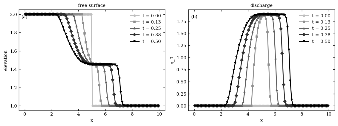
../../../_images/bdea3b938859375627eaa5908d90abf9ae9a9c2a99deddb889a60e6e15ec0380.png

Going further#

One case, one level, no refinement. The maintained end-to-end examples are the AMReX test suite itself — library/zoomy_amrex/tests/ — which builds and runs these same generated headers:

cd library/zoomy_amrex && python3 -m pytest -m small -q

That suite covers a wet dam break (Stoker), a dry one (Ritter), 2-D, a lake-at-rest well-balancing check, NumPy parity, and a two-rank parallel run.

What carries over#

Nothing about the model changed to target AMReX. Swap the last step and the same nsm drives NumPy, JAX, or OpenFOAM — see Backends.